


참고
Go to the end to download the full example code.
PyTorch 프로파일러(Profiler)#
이 레시피에서는 어떻게 PyTorch 프로파일러를 사용하는지, 그리고 모델의 연산자들이 소비하는 메모리와 시간을 측정하는 방법을 살펴보겠습니다.
개요#
PyTorch는 사용자가 모델 내의 연산 비용이 큰(expensive) 연산자들이 무엇인지 알고싶을 때 유용하게 사용할 수 있는 간단한 프로파일러 API를 포함하고 있습니다.
이 레시피에서는 모델의 성능(performance)을 분석하려고 할 때 어떻게 프로파일러를 사용해야 하는지를 보여주기 위해 간단한 ResNet 모델을 사용하겠습니다.
설정(Setup)#
torch 와 torchvision 을 설치하기 위해서 아래의 커맨드를 입력합니다:
pip install torch torchvision
단계(Steps)#
필요한 라이브러리들 불러오기
간단한 ResNet 모델 인스턴스화 하기
프로파일러를 사용하여 실행시간 분석하기
프로파일러를 사용하여 메모리 소비 분석하기
추적기능 사용하기
Examining stack traces
Using profiler to analyze long-running jobs
1. 필요한 라이브러리들 불러오기#
이 레시피에서는 torch 와 torchvision.models,
그리고 profiler 모듈을 사용합니다:
import torch
import torchvision.models as models
from torch.profiler import profile, record_function, ProfilerActivity
2. 간단한 ResNet 모델 인스턴스화 하기#
ResNet 모델 인스턴스를 만들고 입력값을 준비합니다 :
model = models.resnet18()
inputs = torch.randn(5, 3, 224, 224)
3. 프로파일러를 사용하여 실행시간 분석하기#
PyTorch 프로파일러는 컨텍스트 메니저(context manager)를 통해 활성화되고, 여러 매개변수를 받을 수 있습니다. 유용한 몇 가지 매개변수는 다음과 같습니다:
activities- a list of activities to profile:ProfilerActivity.CPU- PyTorch operators, TorchScript functions and user-defined code labels (seerecord_functionbelow);ProfilerActivity.CUDA- on-device CUDA kernels;
record_shapes- 연사자 입력(input)의 shape을 기록할지 여부;profile_memory- 모델의 텐서(Tensor)들이 소비하는 메모리 양을 보고(report)할지 여부;use_cuda- CUDA 커널의 실행시간을 측정할지 여부;
Note: when using CUDA, profiler also shows the runtime CUDA events occuring on the host.
프로파일러를 사용하여 어떻게 실행시간을 분석하는지 보겠습니다:
with profile(activities=[ProfilerActivity.CPU], record_shapes=True) as prof:
    with record_function("model_inference"):
        model(inputs)
record_function 컨텍스트 관리자를 사용하여 임의의 코드 범위에
사용자가 지정한 이름으로 레이블(label)을 표시할 수 있습니다.
(위 예제에서는 model_inference 를 레이블로 사용했습니다.)
프로파일러를 사용하면 프로파일러 컨텍스트 관리자로 감싸진(wrap) 코드 범위를 실행하는 동안 어떤 연산자들이 호출되었는지 확인할 수 있습니다.
만약 여러 프로파일러의 범위가 동시에 활성화된 경우(예. PyTorch 쓰레드가 병렬로
실행 중인 경우), 각 프로파일링 컨텍스트 관리자는 각각의 범위 내의 연산자들만
추적(track)합니다.
프로파일러는 또한 torch.jit._fork 로 실행된 비동기 작업과
(역전파 단계의 경우) backward() 의 호출로 실행된 역전파 연산자들도
자동으로 프로파일링합니다.
위 코드를 실행한 통계를 출력해보겠습니다:
print(prof.key_averages().table(sort_by="cpu_time_total", row_limit=10))
---------------------------------  ------------  ------------  ------------  ------------  ------------  ------------
                             Name    Self CPU %      Self CPU   CPU total %     CPU total  CPU time avg    # of Calls
---------------------------------  ------------  ------------  ------------  ------------  ------------  ------------
                  model_inference         7.18%       3.482ms       100.00%      48.497ms      48.497ms             1
                     aten::conv2d         0.18%      85.560us        77.19%      37.435ms       1.872ms            20
                aten::convolution         0.46%     222.623us        77.01%      37.349ms       1.867ms            20
               aten::_convolution         0.32%     156.516us        76.55%      37.127ms       1.856ms            20
         aten::mkldnn_convolution        75.92%      36.819ms        76.23%      36.970ms       1.849ms            20
                 aten::batch_norm         0.12%      56.538us         9.91%       4.805ms     240.234us            20
     aten::_batch_norm_impl_index         0.23%     110.516us         9.79%       4.748ms     237.407us            20
          aten::native_batch_norm         9.27%       4.494ms         9.54%       4.628ms     231.384us            20
                      aten::relu_         0.39%     187.916us         1.80%     874.065us      51.416us            17
                 aten::max_pool2d         0.05%      26.233us         1.43%     693.791us     693.791us             1
---------------------------------  ------------  ------------  ------------  ------------  ------------  ------------
Self CPU time total: 48.497ms
(몇몇 열을 제외하고) 출력값이 이렇게 보일 것입니다:
- ——————————— ———— ———— ———— ————
Name Self CPU CPU total CPU time avg # of Calls
- ——————————— ———— ———— ———— ————
- model_inference 5.509ms 57.503ms 57.503ms 1
aten::conv2d 231.000us 31.931ms 1.597ms 20
aten::convolution 250.000us 31.700ms 1.585ms 20
aten::_convolution 336.000us 31.450ms 1.573ms 20
- aten::mkldnn_convolution 30.838ms 31.114ms 1.556ms 20
aten::batch_norm 211.000us 14.693ms 734.650us 20
- aten::_batch_norm_impl_index 319.000us 14.482ms 724.100us 20
- aten::native_batch_norm 9.229ms 14.109ms 705.450us 20
aten::mean 332.000us 2.631ms 125.286us 21
aten::select 1.668ms 2.292ms 8.988us 255
——————————— ———— ———— ———— ———— Self CPU time total: 57.549ms
예상했던 대로, 대부분의 시간이 합성곱(convolution) 연산(특히 MKL-DNN 을 지원하도록
컴파일된 PyTorch의 경우에는 mkldnn_convolution )에서 소요되는 것을 확인할 수 있습니다.
(결과 열들 중) Self CPU time과 CPU time의 차이에 유의해야 합니다 -
연산자는 다른 연산자들을 호출할 수 있으며, Self CPU time에는 하위(child) 연산자 호출에서 발생한
시간을 제외해서, Totacl CPU time에는 포함해서 표시합니다.
You can choose to sort by the self cpu time by passing
sort_by="self_cpu_time_total" into the table call.
보다 세부적인 결과 정보 및 연산자의 입력 shape을 함께 보려면 group_by_input_shape=True 를
인자로 전달하면 됩니다
(note: this requires running the profiler with record_shapes=True):
print(prof.key_averages(group_by_input_shape=True).table(sort_by="cpu_time_total", row_limit=10))
---------------------------------  ------------  ------------  ------------  ------------  ------------  ------------  --------------------------------------------------------------------------------
                             Name    Self CPU %      Self CPU   CPU total %     CPU total  CPU time avg    # of Calls                                                                      Input Shapes
---------------------------------  ------------  ------------  ------------  ------------  ------------  ------------  --------------------------------------------------------------------------------
                  model_inference         7.18%       3.482ms       100.00%      48.497ms      48.497ms             1                                                                                []
                     aten::conv2d         0.06%      28.275us        27.06%      13.125ms      13.125ms             1                             [[5, 3, 224, 224], [64, 3, 7, 7], [], [], [], [], []]
                aten::convolution         0.15%      73.125us        27.00%      13.097ms      13.097ms             1                     [[5, 3, 224, 224], [64, 3, 7, 7], [], [], [], [], [], [], []]
               aten::_convolution         0.08%      39.220us        26.85%      13.024ms      13.024ms             1     [[5, 3, 224, 224], [64, 3, 7, 7], [], [], [], [], [], [], [], [], [], [], []]
         aten::mkldnn_convolution        26.70%      12.946ms        26.77%      12.984ms      12.984ms             1                             [[5, 3, 224, 224], [64, 3, 7, 7], [], [], [], [], []]
                     aten::conv2d         0.03%      14.640us        19.12%       9.274ms       2.318ms             4                             [[5, 64, 56, 56], [64, 64, 3, 3], [], [], [], [], []]
                aten::convolution         0.08%      37.078us        19.09%       9.259ms       2.315ms             4                     [[5, 64, 56, 56], [64, 64, 3, 3], [], [], [], [], [], [], []]
               aten::_convolution         0.07%      32.106us        19.02%       9.222ms       2.306ms             4     [[5, 64, 56, 56], [64, 64, 3, 3], [], [], [], [], [], [], [], [], [], [], []]
         aten::mkldnn_convolution        18.90%       9.165ms        18.95%       9.190ms       2.297ms             4                             [[5, 64, 56, 56], [64, 64, 3, 3], [], [], [], [], []]
                     aten::conv2d         0.02%       9.454us         5.14%       2.491ms     830.217us             3                          [[5, 128, 28, 28], [128, 128, 3, 3], [], [], [], [], []]
---------------------------------  ------------  ------------  ------------  ------------  ------------  ------------  --------------------------------------------------------------------------------
Self CPU time total: 48.497ms
(몇몇 열을 제외하고) 출력값이 이렇게 보일 것입니다:
---------------------------------  ------------  -------------------------------------------
                             Name     CPU total                                 Input Shapes
---------------------------------  ------------  -------------------------------------------
                  model_inference      57.503ms                                           []
                     aten::conv2d       8.008ms      [5,64,56,56], [64,64,3,3], [], ..., []]
                aten::convolution       7.956ms     [[5,64,56,56], [64,64,3,3], [], ..., []]
               aten::_convolution       7.909ms     [[5,64,56,56], [64,64,3,3], [], ..., []]
         aten::mkldnn_convolution       7.834ms     [[5,64,56,56], [64,64,3,3], [], ..., []]
                     aten::conv2d       6.332ms    [[5,512,7,7], [512,512,3,3], [], ..., []]
                aten::convolution       6.303ms    [[5,512,7,7], [512,512,3,3], [], ..., []]
               aten::_convolution       6.273ms    [[5,512,7,7], [512,512,3,3], [], ..., []]
         aten::mkldnn_convolution       6.233ms    [[5,512,7,7], [512,512,3,3], [], ..., []]
                     aten::conv2d       4.751ms  [[5,256,14,14], [256,256,3,3], [], ..., []]
---------------------------------  ------------  -------------------------------------------
Self CPU time total: 57.549ms
Note the occurence of aten::convolution twice with different input shapes.
Profiler can also be used to analyze performance of models executed on GPUs:
model = models.resnet18().cuda()
inputs = torch.randn(5, 3, 224, 224).cuda()

with profile(activities=[
        ProfilerActivity.CPU, ProfilerActivity.CUDA], record_shapes=True) as prof:
    with record_function("model_inference"):
        model(inputs)

print(prof.key_averages().table(sort_by="cuda_time_total", row_limit=10))
-------------------------------------------------------  ------------  ------------  ------------  ------------  ------------  ------------  ------------  ------------  ------------  ------------
                                                   Name    Self CPU %      Self CPU   CPU total %     CPU total  CPU time avg     Self CUDA   Self CUDA %    CUDA total  CUDA time avg    # of Calls
-------------------------------------------------------  ------------  ------------  ------------  ------------  ------------  ------------  ------------  ------------  ------------  ------------
                                        model_inference         0.00%       0.000us         0.00%       0.000us       0.000us     175.291ms     26096.35%     175.291ms      87.645ms             2
                                        model_inference         0.61%       1.807ms       100.00%     297.875ms     297.875ms       0.000us         0.00%       2.261ms       2.261ms             1
                                           aten::conv2d         0.02%      62.357us        51.66%     153.899ms       7.695ms       0.000us         0.00%       1.832ms      91.605us            20
                                      aten::convolution         0.06%     183.470us        51.64%     153.837ms       7.692ms       0.000us         0.00%       1.832ms      91.605us            20
                                     aten::_convolution         0.05%     157.311us        51.58%     153.654ms       7.683ms       0.000us         0.00%       1.832ms      91.605us            20
                                aten::cudnn_convolution        38.49%     114.645ms        51.53%     153.496ms       7.675ms     441.244us        65.69%       1.832ms      91.605us            20
                       Runtime Triggered Module Loading        22.26%      66.323ms        22.26%      66.323ms       1.745ms     972.922us       144.84%     972.922us      25.603us            38
                                   cudaFuncSetAttribute         4.97%      14.817ms         5.17%      15.401ms     229.863us       0.000us         0.00%     671.456us      10.022us            67
                                  Lazy Function Loading         0.30%     886.844us         0.30%     886.844us      36.952us     560.986us        83.52%     560.986us      23.374us            24
                                       cudaLaunchKernel         1.70%       5.064ms        19.49%      58.061ms     509.304us       0.000us         0.00%     358.879us       3.148us           114
-------------------------------------------------------  ------------  ------------  ------------  ------------  ------------  ------------  ------------  ------------  ------------  ------------
Self CPU time total: 297.884ms
Self CUDA time total: 671.707us
(Note: the first use of CUDA profiling may bring an extra overhead.)
The resulting table output:
-------------------------------------------------------  ------------  ------------
                                                   Name     Self CUDA    CUDA total
-------------------------------------------------------  ------------  ------------
                                        model_inference       0.000us      11.666ms
                                           aten::conv2d       0.000us      10.484ms
                                      aten::convolution       0.000us      10.484ms
                                     aten::_convolution       0.000us      10.484ms
                             aten::_convolution_nogroup       0.000us      10.484ms
                                      aten::thnn_conv2d       0.000us      10.484ms
                              aten::thnn_conv2d_forward      10.484ms      10.484ms
void at::native::im2col_kernel<float>(long, float co...       3.844ms       3.844ms
                                      sgemm_32x32x32_NN       3.206ms       3.206ms
                                  sgemm_32x32x32_NN_vec       3.093ms       3.093ms
-------------------------------------------------------  ------------  ------------
Self CPU time total: 23.015ms
Self CUDA time total: 11.666ms
Note the occurence of on-device kernels in the output (e.g. sgemm_32x32x32_NN).
4. 프로파일러를 사용하여 메모리 소비 분석하기#
PyTorch 프로파일러는 모델의 연산자들을 실행하며 (모델의 텐서들이 사용하며) 할당(또는 해제)한
메모리의 양도 표시할 수 있습니다.
아래 출력 결과에서 ‘Self’ memory는 해당 연산자에 의해 호출된 하위(child) 연산자들을 제외한,
연산자 자체에 할당(해제)된 메모리에 해당합니다.
메모리 프로파일링 기능을 활성화하려면 profile_memory=True 를 인자로 전달하면 됩니다.
model = models.resnet18()
inputs = torch.randn(5, 3, 224, 224)

with profile(activities=[ProfilerActivity.CPU],
        profile_memory=True, record_shapes=True) as prof:
    model(inputs)

print(prof.key_averages().table(sort_by="self_cpu_memory_usage", row_limit=10))
---------------------------------  ------------  ------------  ------------  ------------  ------------  ------------  ------------  ------------
                             Name    Self CPU %      Self CPU   CPU total %     CPU total  CPU time avg       CPU Mem  Self CPU Mem    # of Calls
---------------------------------  ------------  ------------  ------------  ------------  ------------  ------------  ------------  ------------
                      aten::empty         0.72%     197.288us         0.72%     197.288us       0.986us      94.85 MB      94.85 MB           200
    aten::max_pool2d_with_indices         2.12%     582.848us         2.12%     582.848us     582.848us      11.48 MB      11.48 MB             1
                      aten::addmm         0.25%      69.163us         0.28%      78.173us      78.173us      19.53 KB      19.53 KB             1
                       aten::mean         0.06%      15.605us         0.41%     112.912us     112.912us      10.00 KB       9.99 KB             1
                       aten::div_         0.06%      15.916us         0.12%      32.224us      32.224us           8 B           4 B             1
              aten::empty_strided         0.01%       3.461us         0.01%       3.461us       3.461us           4 B           4 B             1
                     aten::conv2d         0.19%      52.158us        80.22%      22.017ms       1.101ms      47.37 MB           0 B            20
                aten::convolution         0.42%     114.002us        80.03%      21.965ms       1.098ms      47.37 MB           0 B            20
               aten::_convolution         0.29%      80.198us        79.62%      21.851ms       1.093ms      47.37 MB           0 B            20
         aten::mkldnn_convolution        78.93%      21.663ms        79.32%      21.770ms       1.089ms      47.37 MB           0 B            20
---------------------------------  ------------  ------------  ------------  ------------  ------------  ------------  ------------  ------------
Self CPU time total: 27.445ms
(몇몇 열은 제외하였습니다)
- ——————————— ———— ———— ————
Name CPU Mem Self CPU Mem # of Calls
- ——————————— ———— ———— ————
aten::empty 94.79 Mb 94.79 Mb 121
- aten::max_pool2d_with_indices 11.48 Mb 11.48 Mb 1
aten::addmm 19.53 Kb 19.53 Kb 1
- aten::empty_strided 572 b 572 b 25
- aten::resize_ 240 b 240 b 6
aten::abs 480 b 240 b 4 aten::add 160 b 160 b 20
- aten::masked_select 120 b 112 b 1
aten::ne 122 b 53 b 6 aten::eq 60 b 30 b 2
——————————— ———— ———— ———— Self CPU time total: 53.064ms
print(prof.key_averages().table(sort_by="cpu_memory_usage", row_limit=10))
---------------------------------  ------------  ------------  ------------  ------------  ------------  ------------  ------------  ------------
                             Name    Self CPU %      Self CPU   CPU total %     CPU total  CPU time avg       CPU Mem  Self CPU Mem    # of Calls
---------------------------------  ------------  ------------  ------------  ------------  ------------  ------------  ------------  ------------
                      aten::empty         0.72%     197.288us         0.72%     197.288us       0.986us      94.85 MB      94.85 MB           200
                 aten::batch_norm         0.16%      43.403us        12.38%       3.396ms     169.818us      47.41 MB           0 B            20
     aten::_batch_norm_impl_index         0.23%      62.749us        12.22%       3.353ms     167.647us      47.41 MB           0 B            20
          aten::native_batch_norm        11.42%       3.133ms        11.95%       3.281ms     164.045us      47.41 MB     -70.50 KB            20
                     aten::conv2d         0.19%      52.158us        80.22%      22.017ms       1.101ms      47.37 MB           0 B            20
                aten::convolution         0.42%     114.002us        80.03%      21.965ms       1.098ms      47.37 MB           0 B            20
               aten::_convolution         0.29%      80.198us        79.62%      21.851ms       1.093ms      47.37 MB           0 B            20
         aten::mkldnn_convolution        78.93%      21.663ms        79.32%      21.770ms       1.089ms      47.37 MB           0 B            20
                 aten::empty_like         0.10%      28.213us         0.18%      50.287us       2.514us      47.37 MB           0 B            20
                 aten::max_pool2d         0.02%       4.325us         2.14%     587.173us     587.173us      11.48 MB           0 B             1
---------------------------------  ------------  ------------  ------------  ------------  ------------  ------------  ------------  ------------
Self CPU time total: 27.445ms
(몇몇 열을 제외하고) 출력값이 이렇게 보일 것입니다:
- ——————————— ———— ———— ————
Name CPU Mem Self CPU Mem # of Calls
- ——————————— ———— ———— ————
aten::empty 94.79 Mb 94.79 Mb 121
aten::batch_norm 47.41 Mb 0 b 20
- aten::_batch_norm_impl_index 47.41 Mb 0 b 20
- aten::native_batch_norm 47.41 Mb 0 b 20
aten::conv2d 47.37 Mb 0 b 20
aten::convolution 47.37 Mb 0 b 20
aten::_convolution 47.37 Mb 0 b 20
- aten::mkldnn_convolution 47.37 Mb 0 b 20
aten::max_pool2d 11.48 Mb 0 b 1
aten::max_pool2d_with_indices 11.48 Mb 11.48 Mb 1
——————————— ———— ———— ———— Self CPU time total: 53.064ms
5. 추적기능 사용하기#
프로파일링 결과는 .json 형태의 추적 파일(trace file)로 출력할 수 있습니다:
model = models.resnet18().cuda()
inputs = torch.randn(5, 3, 224, 224).cuda()

with profile(activities=[ProfilerActivity.CPU, ProfilerActivity.CUDA]) as prof:
    model(inputs)

prof.export_chrome_trace("trace.json")
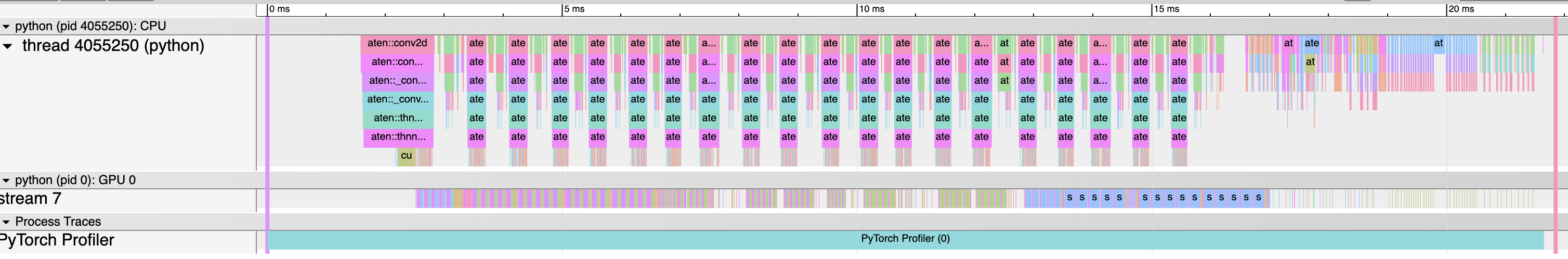
사용자는 Chrome 브라우저( chrome://tracing )에서 추적 파일을 불러와
프로파일된 일련의 연산자들과 CUDA 커널을 검토해볼 수 있습니다:
6. Examining stack traces#
Profiler can be used to analyze Python and TorchScript stack traces:
with profile(
    activities=[ProfilerActivity.CPU, ProfilerActivity.CUDA],
    with_stack=True,
) as prof:
    model(inputs)

# Print aggregated stats
print(prof.key_averages(group_by_stack_n=5).table(sort_by="self_cuda_time_total", row_limit=2))
-------------------------------------------------------  ------------  ------------  ------------  ------------  ------------  ------------  ------------  ------------  ------------  ------------
                                                   Name    Self CPU %      Self CPU   CPU total %     CPU total  CPU time avg     Self CUDA   Self CUDA %    CUDA total  CUDA time avg    # of Calls
-------------------------------------------------------  ------------  ------------  ------------  ------------  ------------  ------------  ------------  ------------  ------------  ------------
                                aten::cudnn_convolution        18.64%     468.092us        40.02%       1.005ms      50.263us     439.095us        65.72%     493.717us      24.686us            20
                                 aten::cudnn_batch_norm        13.65%     342.745us        28.41%     713.615us      35.681us     134.335us        20.11%     134.335us       6.717us            20
-------------------------------------------------------  ------------  ------------  ------------  ------------  ------------  ------------  ------------  ------------  ------------  ------------
Self CPU time total: 2.512ms
Self CUDA time total: 668.110us
The output might look like this (omitting some columns):
-------------------------  -----------------------------------------------------------
                     Name  Source Location
-------------------------  -----------------------------------------------------------
aten::thnn_conv2d_forward  .../torch/nn/modules/conv.py(439): _conv_forward
                           .../torch/nn/modules/conv.py(443): forward
                           .../torch/nn/modules/module.py(1051): _call_impl
                           .../site-packages/torchvision/models/resnet.py(63): forward
                           .../torch/nn/modules/module.py(1051): _call_impl
aten::thnn_conv2d_forward  .../torch/nn/modules/conv.py(439): _conv_forward
                           .../torch/nn/modules/conv.py(443): forward
                           .../torch/nn/modules/module.py(1051): _call_impl
                           .../site-packages/torchvision/models/resnet.py(59): forward
                           .../torch/nn/modules/module.py(1051): _call_impl
-------------------------  -----------------------------------------------------------
Self CPU time total: 34.016ms
Self CUDA time total: 11.659ms
Note the two convolutions and the two call sites in torchvision/models/resnet.py script.
(Warning: stack tracing adds an extra profiling overhead.)
7. Using profiler to analyze long-running jobs#
PyTorch profiler offers an additional API to handle long-running jobs (such as training loops). Tracing all of the execution can be slow and result in very large trace files. To avoid this, use optional arguments:
schedule- specifies a function that takes an integer argument (step number) as an input and returns an action for the profiler, the best way to use this parameter is to usetorch.profiler.schedulehelper function that can generate a schedule for you;on_trace_ready- specifies a function that takes a reference to the profiler as an input and is called by the profiler each time the new trace is ready.
To illustrate how the API works, let’s first consider the following example with
torch.profiler.schedule helper function:
from torch.profiler import schedule

my_schedule = schedule(
    skip_first=10,
    wait=5,
    warmup=1,
    active=3,
    repeat=2)
Profiler assumes that the long-running job is composed of steps, numbered starting from zero. The example above defines the following sequence of actions for the profiler:
Parameter
skip_firsttells profiler that it should ignore the first 10 steps (default value ofskip_firstis zero);After the first
skip_firststeps, profiler starts executing profiler cycles;Each cycle consists of three phases:
idling (
wait=5steps), during this phase profiler is not active;warming up (
warmup=1steps), during this phase profiler starts tracing, but the results are discarded; this phase is used to discard the samples obtained by the profiler at the beginning of the trace since they are usually skewed by an extra overhead;active tracing (
active=3steps), during this phase profiler traces and records data;
An optional
repeatparameter specifies an upper bound on the number of cycles. By default (zero value), profiler will execute cycles as long as the job runs.
Thus, in the example above, profiler will skip the first 15 steps, spend the next step on the warm up,
actively record the next 3 steps, skip another 5 steps, spend the next step on the warm up, actively
record another 3 steps. Since the repeat=2 parameter value is specified, the profiler will stop
the recording after the first two cycles.
At the end of each cycle profiler calls the specified on_trace_ready function and passes itself as
an argument. This function is used to process the new trace - either by obtaining the table output or
by saving the output on disk as a trace file.
To send the signal to the profiler that the next step has started, call prof.step() function.
The current profiler step is stored in prof.step_num.
The following example shows how to use all of the concepts above:
def trace_handler(p):
    output = p.key_averages().table(sort_by="self_cuda_time_total", row_limit=10)
    print(output)
    p.export_chrome_trace("/tmp/trace_" + str(p.step_num) + ".json")

with profile(
    activities=[ProfilerActivity.CPU, ProfilerActivity.CUDA],
    schedule=torch.profiler.schedule(
        wait=1,
        warmup=1,
        active=2),
    on_trace_ready=trace_handler
) as p:
    for idx in range(8):
        model(inputs)
        p.step()
-------------------------------------------------------  ------------  ------------  ------------  ------------  ------------  ------------  ------------  ------------  ------------  ------------
                                                   Name    Self CPU %      Self CPU   CPU total %     CPU total  CPU time avg     Self CUDA   Self CUDA %    CUDA total  CUDA time avg    # of Calls
-------------------------------------------------------  ------------  ------------  ------------  ------------  ------------  ------------  ------------  ------------  ------------  ------------
                                          ProfilerStep*         0.00%       0.000us         0.00%       0.000us       0.000us       5.280ms       395.25%       5.280ms       2.640ms             2
                                aten::cudnn_convolution        13.41%     755.975us        24.93%       1.405ms      35.128us     878.128us        65.74%     878.128us      21.953us            40
                                 aten::cudnn_batch_norm        10.72%     604.499us        22.93%       1.293ms      32.316us     269.951us        20.21%     269.951us       6.749us            40
void cudnn::bn_fw_tr_1C11_singleread<float, 512, tru...         0.00%       0.000us         0.00%       0.000us       0.000us     212.735us        15.93%     212.735us       5.598us            38
void cudnn::engines_precompiled::nchwToNhwcKernel<fl...         0.00%       0.000us         0.00%       0.000us       0.000us     194.492us        14.56%     194.492us       4.862us            40
sm80_xmma_fprop_implicit_gemm_tf32f32_tf32f32_f32_nh...         0.00%       0.000us         0.00%       0.000us       0.000us     135.548us        10.15%     135.548us      16.944us             8
sm90_xmma_fprop_implicit_gemm_f32f32_tf32f32_f32_nhw...         0.00%       0.000us         0.00%       0.000us       0.000us     115.100us         8.62%     115.100us      11.510us            10
sm80_xmma_fprop_implicit_gemm_tf32f32_tf32f32_f32_nh...         0.00%       0.000us         0.00%       0.000us       0.000us     112.512us         8.42%     112.512us      11.251us            10
void cudnn::engines_precompiled::nchwToNhwcKernel<fl...         0.00%       0.000us         0.00%       0.000us       0.000us      88.960us         6.66%      88.960us       2.780us            32
                                             aten::add_         4.31%     242.683us         7.96%     448.469us       8.008us      73.633us         5.51%      73.633us       1.315us            56
-------------------------------------------------------  ------------  ------------  ------------  ------------  ------------  ------------  ------------  ------------  ------------  ------------
Self CPU time total: 5.637ms
Self CUDA time total: 1.336ms

-------------------------------------------------------  ------------  ------------  ------------  ------------  ------------  ------------  ------------  ------------  ------------  ------------
                                                   Name    Self CPU %      Self CPU   CPU total %     CPU total  CPU time avg     Self CUDA   Self CUDA %    CUDA total  CUDA time avg    # of Calls
-------------------------------------------------------  ------------  ------------  ------------  ------------  ------------  ------------  ------------  ------------  ------------  ------------
                                          ProfilerStep*         0.00%       0.000us         0.00%       0.000us       0.000us       5.249ms       392.52%       5.249ms       2.624ms             2
                                aten::cudnn_convolution        13.66%     765.311us        25.29%       1.417ms      35.434us     880.464us        65.85%     880.464us      22.012us            40
                                 aten::cudnn_batch_norm        10.65%     597.080us        22.96%       1.287ms      32.170us     269.596us        20.16%     269.596us       6.740us            40
void cudnn::bn_fw_tr_1C11_singleread<float, 512, tru...         0.00%       0.000us         0.00%       0.000us       0.000us     212.060us        15.86%     212.060us       5.581us            38
void cudnn::engines_precompiled::nchwToNhwcKernel<fl...         0.00%       0.000us         0.00%       0.000us       0.000us     195.386us        14.61%     195.386us       4.885us            40
sm80_xmma_fprop_implicit_gemm_tf32f32_tf32f32_f32_nh...         0.00%       0.000us         0.00%       0.000us       0.000us     136.638us        10.22%     136.638us      17.080us             8
sm90_xmma_fprop_implicit_gemm_f32f32_tf32f32_f32_nhw...         0.00%       0.000us         0.00%       0.000us       0.000us     114.590us         8.57%     114.590us      11.459us            10
sm80_xmma_fprop_implicit_gemm_tf32f32_tf32f32_f32_nh...         0.00%       0.000us         0.00%       0.000us       0.000us     112.766us         8.43%     112.766us      11.277us            10
void cudnn::engines_precompiled::nchwToNhwcKernel<fl...         0.00%       0.000us         0.00%       0.000us       0.000us      88.672us         6.63%      88.672us       2.771us            32
                                             aten::add_         4.35%     243.530us         8.14%     456.116us       8.145us      73.252us         5.48%      73.252us       1.308us            56
-------------------------------------------------------  ------------  ------------  ------------  ------------  ------------  ------------  ------------  ------------  ------------  ------------
Self CPU time total: 5.604ms
Self CUDA time total: 1.337ms
더 알아보기#
다음 레시피와 튜토리얼을 읽으며 학습을 계속해보세요:
Total running time of the script: (0 minutes 3.909 seconds)
