


참고
Go to the end to download the full example code.
wav2vec2을 이용한 강제 정렬#
이번 튜토리얼에서는 CTC-Segmentation of Large Corpora for German End-to-end Speech Recognition 에서 설명한 CTC 분할 알고리즘을 이용하여 torchaudio를 가지고 정답 스크립트를 음성에 맞추는 방법에 대해 설명합니다.
참고
이 튜토리얼은 원래 Wav2Vec2의 사용 사례를 설명하기 위해 작성되었습니다.
TorchAudio에는 강제 정렬을 위해 설계된 API가 있습니다.
CTC forced alignment API tutorial 은 핵심 API인
torchaudio.functional.forced_align() 의 사용법에 대해 보여주고 있습니다.
만약 본인만의 코퍼스에 대해 강제 정렬하려는 경우, torchaudio.pipelines.Wav2Vec2FABundle 를 사용하는 것을 추천합니다.
이는 강제 정렬을 위해 특별히 훈련된 사전 훈련 모델과 함께 forced_align() 및 여러 함수를 결합하여 사용할 수 있게 합니다.
사용법에 대한 자세한 내용은 다국어 데이터를 위한 강제 정렬을 설명하는 Forced alignment for multilingual data 를 참조하세요.
import torch
import torchaudio

print(torch.__version__)
print(torchaudio.__version__)


device = torch.device("cuda" if torch.cuda.is_available() else "cpu")
print(device)
2.8.0+cu128
2.8.0+cu128
cuda
개요#
정렬 과정은 다음과 같습니다.
오디오 파형으로부터 프레임별 라벨 확률을 추정한다.
각 시간 별로 정렬된 라벨의 확률을 나타내는 trellis 행렬을 생성한다.
trellis 행렬로부터 가장 가능성이 높은 경로를 찾는다.
이번 예시에는 음성 특징 추출을 위해 torchaudio의 wav2vec2 모델을 사용합니다.
준비#
먼저 필요한 패키지를 임포트하고, 작업할 데이터를 불러옵니다.
from dataclasses import dataclass

import IPython
import matplotlib.pyplot as plt

torch.random.manual_seed(0)

SPEECH_FILE = torchaudio.utils.download_asset("tutorial-assets/Lab41-SRI-VOiCES-src-sp0307-ch127535-sg0042.wav")
/workspace/tutorials-kr/intermediate_source/forced_alignment_with_torchaudio_tutorial.py:62: UserWarning:

torchaudio.utils.download.download_asset has been deprecated. This deprecation is part of a large refactoring effort to transition TorchAudio into a maintenance phase. Please see https://github.com/pytorch/audio/issues/3902 for more information. It will be removed from the 2.9 release.


  0%|          | 0.00/106k [00:00<?, ?B/s]
100%|██████████| 106k/106k [00:00<00:00, 17.1MB/s]
프레임 별 라벨 확률 생성#
첫번째 과정은 각 오디오 프레임 별 라벨 클래스 확률을 생성하는 것입니다.
ASR(음성 인식)용으로 학습된 wav2vec2 모델을 사용할 수 있습니다.
여기서는 torchaudio.pipelines.WAV2VEC2_ASR_BASE_960H() 를 사용합니다.
``torchaudio``는 연관된 라벨과 함께 미리 학습된 모델에 쉽게 접근할 수 있게 합니다.
참고
여기서는 수치적인 불안정성을 피하고자 로그 도메인에서 확률을 계산할 것입니다.
이렇게 하기 위해 torch.log_softmax() 를 사용하여 출력 확률 을 정규화합니다.
bundle = torchaudio.pipelines.WAV2VEC2_ASR_BASE_960H
model = bundle.get_model().to(device)
labels = bundle.get_labels()
with torch.inference_mode():
    waveform, _ = torchaudio.load(SPEECH_FILE)
    emissions, _ = model(waveform.to(device))
    emissions = torch.log_softmax(emissions, dim=-1)

emission = emissions[0].cpu().detach()

print(labels)
Downloading: "https://download.pytorch.org/torchaudio/models/wav2vec2_fairseq_base_ls960_asr_ls960.pth" to /root/.cache/torch/hub/checkpoints/wav2vec2_fairseq_base_ls960_asr_ls960.pth

  0%|          | 0.00/360M [00:00<?, ?B/s]
  1%|▏         | 5.25M/360M [00:00<00:06, 55.0MB/s]
  4%|▍         | 15.0M/360M [00:00<00:04, 82.5MB/s]
  7%|▋         | 25.5M/360M [00:00<00:03, 94.8MB/s]
 10%|█         | 36.4M/360M [00:00<00:03, 102MB/s]
 13%|█▎        | 47.5M/360M [00:00<00:03, 107MB/s]
 16%|█▋        | 58.6M/360M [00:00<00:02, 110MB/s]
 19%|█▉        | 69.2M/360M [00:00<00:02, 110MB/s]
 22%|██▏       | 80.0M/360M [00:00<00:02, 111MB/s]
 25%|██▌       | 91.0M/360M [00:00<00:02, 112MB/s]
 29%|██▊       | 103M/360M [00:01<00:02, 117MB/s]
 32%|███▏      | 114M/360M [00:01<00:02, 113MB/s]
 35%|███▍      | 125M/360M [00:01<00:02, 113MB/s]
 38%|███▊      | 136M/360M [00:01<00:02, 114MB/s]
 41%|████▏     | 149M/360M [00:01<00:01, 118MB/s]
 44%|████▍     | 160M/360M [00:01<00:01, 113MB/s]
 48%|████▊     | 171M/360M [00:01<00:01, 114MB/s]
 51%|█████     | 182M/360M [00:01<00:01, 114MB/s]
 54%|█████▎    | 193M/360M [00:01<00:01, 114MB/s]
 57%|█████▋    | 204M/360M [00:01<00:01, 115MB/s]
 60%|█████▉    | 216M/360M [00:02<00:01, 112MB/s]
 63%|██████▎   | 226M/360M [00:02<00:01, 109MB/s]
 66%|██████▌   | 237M/360M [00:02<00:01, 105MB/s]
 69%|██████▊   | 247M/360M [00:02<00:01, 101MB/s]
 71%|███████▏  | 257M/360M [00:02<00:01, 95.2MB/s]
 74%|███████▍  | 266M/360M [00:02<00:01, 89.9MB/s]
 76%|███████▌  | 275M/360M [00:02<00:01, 87.8MB/s]
 79%|███████▊  | 283M/360M [00:02<00:00, 86.7MB/s]
 81%|████████  | 292M/360M [00:02<00:00, 87.1MB/s]
 83%|████████▎ | 300M/360M [00:03<00:00, 87.2MB/s]
 86%|████████▌ | 308M/360M [00:03<00:00, 84.4MB/s]
 88%|████████▊ | 318M/360M [00:03<00:00, 89.2MB/s]
 91%|█████████ | 328M/360M [00:03<00:00, 94.0MB/s]
 94%|█████████▍| 338M/360M [00:03<00:00, 95.5MB/s]
 97%|█████████▋| 349M/360M [00:03<00:00, 101MB/s]
100%|██████████| 360M/360M [00:03<00:00, 106MB/s]
100%|██████████| 360M/360M [00:03<00:00, 103MB/s]
/opt/conda/lib/python3.11/site-packages/torchaudio/_backend/utils.py:213: UserWarning:

In 2.9, this function's implementation will be changed to use torchaudio.load_with_torchcodec` under the hood. Some parameters like ``normalize``, ``format``, ``buffer_size``, and ``backend`` will be ignored. We recommend that you port your code to rely directly on TorchCodec's decoder instead: https://docs.pytorch.org/torchcodec/stable/generated/torchcodec.decoders.AudioDecoder.html#torchcodec.decoders.AudioDecoder.

/opt/conda/lib/python3.11/site-packages/torchaudio/_backend/ffmpeg.py:88: UserWarning:

torio.io._streaming_media_decoder.StreamingMediaDecoder has been deprecated. This deprecation is part of a large refactoring effort to transition TorchAudio into a maintenance phase. The decoding and encoding capabilities of PyTorch for both audio and video are being consolidated into TorchCodec. Please see https://github.com/pytorch/audio/issues/3902 for more information. It will be removed from the 2.9 release.

('-', '|', 'E', 'T', 'A', 'O', 'N', 'I', 'H', 'S', 'R', 'D', 'L', 'U', 'M', 'W', 'C', 'F', 'G', 'Y', 'P', 'B', 'V', 'K', "'", 'X', 'J', 'Q', 'Z')
시각화#
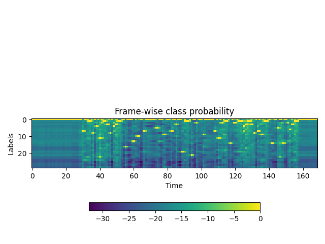
def plot():
    fig, ax = plt.subplots()
    img = ax.imshow(emission.T)
    ax.set_title("Frame-wise class probability")
    ax.set_xlabel("Time")
    ax.set_ylabel("Labels")
    fig.colorbar(img, ax=ax, shrink=0.6, location="bottom")
    fig.tight_layout()


plot()
정렬 확률 생성 (trellis)#
다음, 출력 행렬로부터 각 프레임에서 정답 스크립트의 라벨들이 등장할 수 있는 확률을 나타내는 trellis를 생성합니다. Trellis는 시간 축과 라벨 축을 가지고 있는 2D 행렬입니다. 라벨 축은 정렬하려는 정답 스크립트를 나타냅니다. \(t\) 를 시간 축에서의 인덱스로 나타내는 데 사용하고, \(j\) 를 라벨 축에서의 인덱스로 나타내는 데 사용합니다. \(c_j\) 는 라벨 인덱스 \(j\) 에서의 라벨을 나타냅니다.
\(t+1\) 시점에서의 확률을 생성하기 위해, \(t\) 시점에서의 trellis와 \(t+1\) 시점에서의 출력을 봅니다. \(t+1\) 시점에서 \(c_{j+1}\) 라벨에 도달할 수 있는 2개의 경로가 있습니다. 첫번째는 \(t\) 시점에서 라벨은 \(c_{j+1}\) 였으며 \(t\) 에서 \({t+1}\) 으로 바뀔 때 라벨 변화는 없는 경우입니다. 다른 경우는 \(t\) 시점에서 라벨은 \(c_j\) 였으며 \(t+1\) 시점에서는 다음 라벨 \(c_{j+1}\) 로 전이된 경우입니다.
아래 그림은 2가지 전이를 나타내고 있습니다.
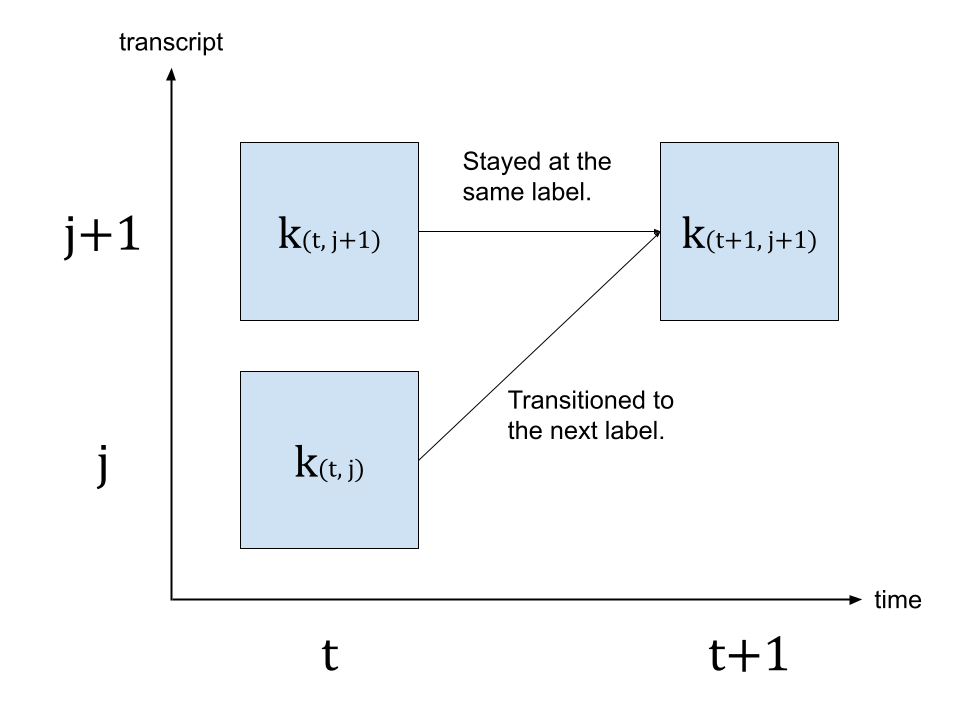
가장 가능성 있는 전이를 찾기 위해, \(k_{(t+1, j+1)}\) 의 값의 가장 가능성 있는 경로를 택합니다. 이는 아래에 나와 있는 식으로 나타낼 수 있습니다.
\(k_{(t+1, j+1)} = max( k_{(t, j)} p(t+1, c_{j+1}), k_{(t, j+1)} p(t+1, repeat) )\)
\(k\) 는 trellis 행렬을 나타내며, \(p(t, c_j)\) 는 \(t\) 시점에서의 라벨 \(c_j\) 의 확률을 나타냅니다. repeat는 CTC 식에서의 블랭크 토큰을 나타냅니다. (CTC 알고리즘에 대한 자세한 설명은 ‘Sequence Modeling with CTC’를 참고하세요.) [distill.pub])
# SOS와 EOS를 나타내는 space 토큰을 가지고 정답 스크립트를 둘러쌈.
transcript = "|I|HAD|THAT|CURIOSITY|BESIDE|ME|AT|THIS|MOMENT|"
dictionary = {c: i for i, c in enumerate(labels)}

tokens = [dictionary[c] for c in transcript]
print(list(zip(transcript, tokens)))


def get_trellis(emission, tokens, blank_id=0):
    num_frame = emission.size(0)
    num_tokens = len(tokens)

    trellis = torch.zeros((num_frame, num_tokens))
    trellis[1:, 0] = torch.cumsum(emission[1:, blank_id], 0)
    trellis[0, 1:] = -float("inf")
    trellis[-num_tokens + 1 :, 0] = float("inf")

    for t in range(num_frame - 1):
        trellis[t + 1, 1:] = torch.maximum(
            # 같은 토큰에 머무르고 있는 경우의 점수
            trellis[t, 1:] + emission[t, blank_id],
            # 다음 토큰으로 바뀌는 경우에 대한 점수
            trellis[t, :-1] + emission[t, tokens[1:]],
        )
    return trellis


trellis = get_trellis(emission, tokens)
[('|', 1), ('I', 7), ('|', 1), ('H', 8), ('A', 4), ('D', 11), ('|', 1), ('T', 3), ('H', 8), ('A', 4), ('T', 3), ('|', 1), ('C', 16), ('U', 13), ('R', 10), ('I', 7), ('O', 5), ('S', 9), ('I', 7), ('T', 3), ('Y', 19), ('|', 1), ('B', 21), ('E', 2), ('S', 9), ('I', 7), ('D', 11), ('E', 2), ('|', 1), ('M', 14), ('E', 2), ('|', 1), ('A', 4), ('T', 3), ('|', 1), ('T', 3), ('H', 8), ('I', 7), ('S', 9), ('|', 1), ('M', 14), ('O', 5), ('M', 14), ('E', 2), ('N', 6), ('T', 3), ('|', 1)]
시각화#
def plot():
    fig, ax = plt.subplots()
    img = ax.imshow(trellis.T, origin="lower")
    ax.annotate("- Inf", (trellis.size(1) / 5, trellis.size(1) / 1.5))
    ax.annotate("+ Inf", (trellis.size(0) - trellis.size(1) / 5, trellis.size(1) / 3))
    fig.colorbar(img, ax=ax, shrink=0.6, location="bottom")
    fig.tight_layout()


plot()
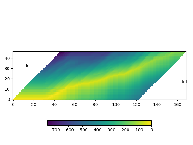
위 시각화된 그림에서, 행렬을 대각선으로 가로지르는 높은 확률의 추적(trace)를 볼 수 있습니다.
가장 가능성 높은 경로 찾기 (백트래킹)#
trellis가 한번 생성되면, 높은 확률을 가지는 요소를 따라 이를 탐색할 수 있습니다.
가장 높은 확률을 가지는 시간 단계에서 마지막 라벨 인덱스로부터 시작합니다. 그 후에, 이전 전이 확률 \(k_{t, j} p(t+1, c_{j+1})\) 또는 \(k_{t, j+1} p(t+1, repeat)`에 기반하여 머무를지 (:math:`c_j \rightarrow c_j\)) 또는 전이할지 (\(c_j \rightarrow c_{j+1}\))를 시간 역순으로 진행합니다.
라벨이 한번 시작 부분에 도달하게 되면, 전이가 수행됩니다.
trellis 행렬은 경로를 찾기 위해 사용되지만, 각 분할의 최종 확률에 대해서는 출력 행렬에서의 프레임별 확률을 사용합니다.
@dataclass
class Point:
    token_index: int
    time_index: int
    score: float


def backtrack(trellis, emission, tokens, blank_id=0):
    t, j = trellis.size(0) - 1, trellis.size(1) - 1

    path = [Point(j, t, emission[t, blank_id].exp().item())]
    while j > 0:
        # 발생하지 않는 경우지만, 혹시 몰라 예외 처리함.
        assert t > 0

        # 1. 현재 위치가 stay인지 또는 change인지를 판단함.
        # stay 대 change의 프레임 별 점수 계산
        p_stay = emission[t - 1, blank_id]
        p_change = emission[t - 1, tokens[j]]

        # stay 대 change의 문맥을 고려한 점수 계산
        stayed = trellis[t - 1, j] + p_stay
        changed = trellis[t - 1, j - 1] + p_change

        # 위치 갱신
        t -= 1
        if changed > stayed:
            j -= 1

        # 프레임별 확률을 이용하여 경로를 저장함.
        prob = (p_change if changed > stayed else p_stay).exp().item()
        path.append(Point(j, t, prob))

    # 지금 j == 0이라면 이는, SoS를 도달했다는 것을 의미함.
    # 시각화를 위해 나머지 부분을 채움.
    while t > 0:
        prob = emission[t - 1, blank_id].exp().item()
        path.append(Point(j, t - 1, prob))
        t -= 1

    return path[::-1]


path = backtrack(trellis, emission, tokens)
for p in path:
    print(p)
Point(token_index=0, time_index=0, score=0.9999996423721313)
Point(token_index=0, time_index=1, score=0.9999996423721313)
Point(token_index=0, time_index=2, score=0.9999996423721313)
Point(token_index=0, time_index=3, score=0.9999996423721313)
Point(token_index=0, time_index=4, score=0.9999996423721313)
Point(token_index=0, time_index=5, score=0.9999996423721313)
Point(token_index=0, time_index=6, score=0.9999996423721313)
Point(token_index=0, time_index=7, score=0.9999996423721313)
Point(token_index=0, time_index=8, score=0.9999998807907104)
Point(token_index=0, time_index=9, score=0.9999996423721313)
Point(token_index=0, time_index=10, score=0.9999996423721313)
Point(token_index=0, time_index=11, score=0.9999998807907104)
Point(token_index=0, time_index=12, score=0.9999996423721313)
Point(token_index=0, time_index=13, score=0.9999996423721313)
Point(token_index=0, time_index=14, score=0.9999996423721313)
Point(token_index=0, time_index=15, score=0.9999996423721313)
Point(token_index=0, time_index=16, score=0.9999996423721313)
Point(token_index=0, time_index=17, score=0.9999996423721313)
Point(token_index=0, time_index=18, score=0.9999998807907104)
Point(token_index=0, time_index=19, score=0.9999996423721313)
Point(token_index=0, time_index=20, score=0.9999996423721313)
Point(token_index=0, time_index=21, score=0.9999996423721313)
Point(token_index=0, time_index=22, score=0.9999996423721313)
Point(token_index=0, time_index=23, score=0.9999997615814209)
Point(token_index=0, time_index=24, score=0.9999998807907104)
Point(token_index=0, time_index=25, score=0.9999998807907104)
Point(token_index=0, time_index=26, score=0.9999998807907104)
Point(token_index=0, time_index=27, score=0.9999998807907104)
Point(token_index=0, time_index=28, score=0.9999985694885254)
Point(token_index=0, time_index=29, score=0.9999943971633911)
Point(token_index=0, time_index=30, score=0.9999842643737793)
Point(token_index=1, time_index=31, score=0.9845577478408813)
Point(token_index=1, time_index=32, score=0.9999706745147705)
Point(token_index=1, time_index=33, score=0.15365149080753326)
Point(token_index=1, time_index=34, score=0.9999173879623413)
Point(token_index=2, time_index=35, score=0.6086527705192566)
Point(token_index=2, time_index=36, score=0.9997723698616028)
Point(token_index=3, time_index=37, score=0.9997126460075378)
Point(token_index=3, time_index=38, score=0.9999358654022217)
Point(token_index=4, time_index=39, score=0.98616623878479)
Point(token_index=4, time_index=40, score=0.9242105484008789)
Point(token_index=5, time_index=41, score=0.9259880185127258)
Point(token_index=5, time_index=42, score=0.015578599646687508)
Point(token_index=5, time_index=43, score=0.9998377561569214)
Point(token_index=6, time_index=44, score=0.9988479614257812)
Point(token_index=7, time_index=45, score=0.10202880948781967)
Point(token_index=7, time_index=46, score=0.9999427795410156)
Point(token_index=8, time_index=47, score=0.9999943971633911)
Point(token_index=8, time_index=48, score=0.9979603290557861)
Point(token_index=9, time_index=49, score=0.036029838025569916)
Point(token_index=9, time_index=50, score=0.061661187559366226)
Point(token_index=9, time_index=51, score=4.3364110752008855e-05)
Point(token_index=10, time_index=52, score=0.9999799728393555)
Point(token_index=11, time_index=53, score=0.9966963529586792)
Point(token_index=11, time_index=54, score=0.9999257326126099)
Point(token_index=11, time_index=55, score=0.9999982118606567)
Point(token_index=12, time_index=56, score=0.9990673661231995)
Point(token_index=12, time_index=57, score=0.9999996423721313)
Point(token_index=12, time_index=58, score=0.9999996423721313)
Point(token_index=12, time_index=59, score=0.8456599712371826)
Point(token_index=12, time_index=60, score=0.9999996423721313)
Point(token_index=13, time_index=61, score=0.999601423740387)
Point(token_index=13, time_index=62, score=0.999998927116394)
Point(token_index=14, time_index=63, score=0.0035245749168097973)
Point(token_index=14, time_index=64, score=1.0)
Point(token_index=14, time_index=65, score=1.0)
Point(token_index=14, time_index=66, score=0.9999915361404419)
Point(token_index=15, time_index=67, score=0.9971538782119751)
Point(token_index=15, time_index=68, score=0.9999990463256836)
Point(token_index=15, time_index=69, score=0.9999992847442627)
Point(token_index=15, time_index=70, score=0.9999997615814209)
Point(token_index=15, time_index=71, score=0.9999998807907104)
Point(token_index=15, time_index=72, score=0.9999881982803345)
Point(token_index=15, time_index=73, score=0.011425581760704517)
Point(token_index=15, time_index=74, score=0.9999977350234985)
Point(token_index=16, time_index=75, score=0.9996119737625122)
Point(token_index=16, time_index=76, score=0.999998927116394)
Point(token_index=16, time_index=77, score=0.9728821516036987)
Point(token_index=16, time_index=78, score=0.999998927116394)
Point(token_index=17, time_index=79, score=0.994936466217041)
Point(token_index=17, time_index=80, score=0.999998927116394)
Point(token_index=17, time_index=81, score=0.9999123811721802)
Point(token_index=17, time_index=82, score=0.9999774694442749)
Point(token_index=18, time_index=83, score=0.6569597125053406)
Point(token_index=18, time_index=84, score=0.9984305500984192)
Point(token_index=18, time_index=85, score=0.9999876022338867)
Point(token_index=19, time_index=86, score=0.9993755221366882)
Point(token_index=19, time_index=87, score=0.9999988079071045)
Point(token_index=19, time_index=88, score=0.1040310338139534)
Point(token_index=19, time_index=89, score=0.9999969005584717)
Point(token_index=20, time_index=90, score=0.39741814136505127)
Point(token_index=20, time_index=91, score=0.9999932050704956)
Point(token_index=21, time_index=92, score=1.6994663383229636e-06)
Point(token_index=21, time_index=93, score=0.9861478209495544)
Point(token_index=21, time_index=94, score=0.9999960660934448)
Point(token_index=22, time_index=95, score=0.9992735981941223)
Point(token_index=22, time_index=96, score=0.999340832233429)
Point(token_index=22, time_index=97, score=0.9999983310699463)
Point(token_index=23, time_index=98, score=0.9999971389770508)
Point(token_index=23, time_index=99, score=0.9999998807907104)
Point(token_index=23, time_index=100, score=0.9999995231628418)
Point(token_index=23, time_index=101, score=0.9999732971191406)
Point(token_index=24, time_index=102, score=0.9983208775520325)
Point(token_index=24, time_index=103, score=0.9999991655349731)
Point(token_index=24, time_index=104, score=0.9999996423721313)
Point(token_index=24, time_index=105, score=0.9999998807907104)
Point(token_index=24, time_index=106, score=1.0)
Point(token_index=24, time_index=107, score=0.9998630285263062)
Point(token_index=24, time_index=108, score=0.9999980926513672)
Point(token_index=25, time_index=109, score=0.9988538026809692)
Point(token_index=25, time_index=110, score=0.9999798536300659)
Point(token_index=26, time_index=111, score=0.8572901487350464)
Point(token_index=26, time_index=112, score=0.9999847412109375)
Point(token_index=27, time_index=113, score=0.9870244264602661)
Point(token_index=27, time_index=114, score=1.9012284610653296e-05)
Point(token_index=27, time_index=115, score=0.9999796152114868)
Point(token_index=28, time_index=116, score=0.9998252391815186)
Point(token_index=28, time_index=117, score=0.9999990463256836)
Point(token_index=29, time_index=118, score=0.9999732971191406)
Point(token_index=29, time_index=119, score=0.0008801211952231824)
Point(token_index=29, time_index=120, score=0.999330461025238)
Point(token_index=30, time_index=121, score=0.9975368976593018)
Point(token_index=30, time_index=122, score=0.00030387210426852107)
Point(token_index=30, time_index=123, score=0.9999344348907471)
Point(token_index=31, time_index=124, score=6.092021521908464e-06)
Point(token_index=31, time_index=125, score=0.9833189249038696)
Point(token_index=32, time_index=126, score=0.9974585175514221)
Point(token_index=33, time_index=127, score=0.0008255028515122831)
Point(token_index=33, time_index=128, score=0.996514618396759)
Point(token_index=34, time_index=129, score=0.017437921836972237)
Point(token_index=34, time_index=130, score=0.9989172220230103)
Point(token_index=35, time_index=131, score=0.9999697208404541)
Point(token_index=36, time_index=132, score=0.9999842643737793)
Point(token_index=36, time_index=133, score=0.9997640252113342)
Point(token_index=37, time_index=134, score=0.5103023648262024)
Point(token_index=37, time_index=135, score=0.9998301267623901)
Point(token_index=38, time_index=136, score=0.08520788699388504)
Point(token_index=38, time_index=137, score=0.004072219133377075)
Point(token_index=38, time_index=138, score=0.9999815225601196)
Point(token_index=39, time_index=139, score=0.012034696526825428)
Point(token_index=39, time_index=140, score=0.9999980926513672)
Point(token_index=39, time_index=141, score=0.0005803863750770688)
Point(token_index=39, time_index=142, score=0.9999070167541504)
Point(token_index=40, time_index=143, score=0.9999960660934448)
Point(token_index=40, time_index=144, score=0.9999980926513672)
Point(token_index=40, time_index=145, score=0.9999916553497314)
Point(token_index=41, time_index=146, score=0.9971185922622681)
Point(token_index=41, time_index=147, score=0.9981784820556641)
Point(token_index=41, time_index=148, score=0.9999310970306396)
Point(token_index=42, time_index=149, score=0.9879414439201355)
Point(token_index=42, time_index=150, score=0.9997634291648865)
Point(token_index=42, time_index=151, score=0.9999536275863647)
Point(token_index=43, time_index=152, score=0.9999715089797974)
Point(token_index=44, time_index=153, score=0.3179967701435089)
Point(token_index=44, time_index=154, score=0.9997820258140564)
Point(token_index=45, time_index=155, score=0.01602203957736492)
Point(token_index=45, time_index=156, score=0.999901294708252)
Point(token_index=46, time_index=157, score=0.46667248010635376)
Point(token_index=46, time_index=158, score=0.9999994039535522)
Point(token_index=46, time_index=159, score=0.9999996423721313)
Point(token_index=46, time_index=160, score=0.9999995231628418)
Point(token_index=46, time_index=161, score=0.9999996423721313)
Point(token_index=46, time_index=162, score=0.9999996423721313)
Point(token_index=46, time_index=163, score=0.9999996423721313)
Point(token_index=46, time_index=164, score=0.9999995231628418)
Point(token_index=46, time_index=165, score=0.9999995231628418)
Point(token_index=46, time_index=166, score=0.9999996423721313)
Point(token_index=46, time_index=167, score=0.9999996423721313)
Point(token_index=46, time_index=168, score=0.9999995231628418)
시각화#
def plot_trellis_with_path(trellis, path):
    # 경로와 함께 trellis를 그리기 위해, 'nan' 값을 이용합니다.
    trellis_with_path = trellis.clone()
    for _, p in enumerate(path):
        trellis_with_path[p.time_index, p.token_index] = float("nan")
    plt.imshow(trellis_with_path.T, origin="lower")
    plt.title("The path found by backtracking")
    plt.tight_layout()


plot_trellis_with_path(trellis, path)
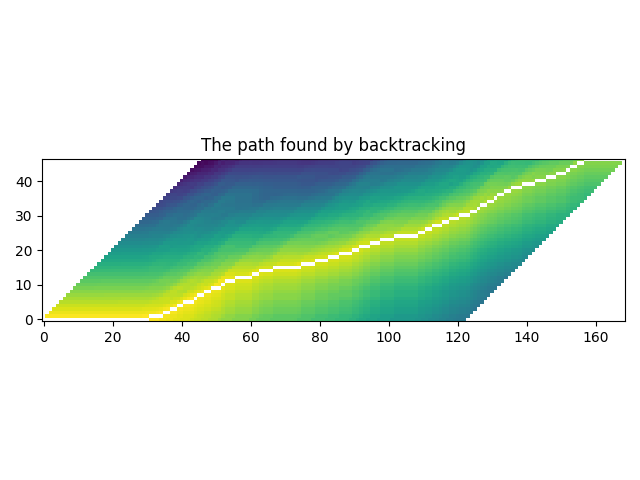
좋습니다.
경로 분할#
지금 이 경로는 같은 라벨의 반복이 포함되어 있기 때문에 이를 병합하여 원본 정답 스크립트와 가깝게 만들어봅시다.
다수의 경로 지점들을 병합할 때 단순하게, 병합된 분할의 평균 확률을 취합니다.
# 라벨을 병합함
@dataclass
class Segment:
    label: str
    start: int
    end: int
    score: float

    def __repr__(self):
        return f"{self.label}\t({self.score:4.2f}): [{self.start:5d}, {self.end:5d})"

    @property
    def length(self):
        return self.end - self.start


def merge_repeats(path):
    i1, i2 = 0, 0
    segments = []
    while i1 < len(path):
        while i2 < len(path) and path[i1].token_index == path[i2].token_index:
            i2 += 1
        score = sum(path[k].score for k in range(i1, i2)) / (i2 - i1)
        segments.append(
            Segment(
                transcript[path[i1].token_index],
                path[i1].time_index,
                path[i2 - 1].time_index + 1,
                score,
            )
        )
        i1 = i2
    return segments


segments = merge_repeats(path)
for seg in segments:
    print(seg)
|       (1.00): [    0,    31)
I       (0.78): [   31,    35)
|       (0.80): [   35,    37)
H       (1.00): [   37,    39)
A       (0.96): [   39,    41)
D       (0.65): [   41,    44)
|       (1.00): [   44,    45)
T       (0.55): [   45,    47)
H       (1.00): [   47,    49)
A       (0.03): [   49,    52)
T       (1.00): [   52,    53)
|       (1.00): [   53,    56)
C       (0.97): [   56,    61)
U       (1.00): [   61,    63)
R       (0.75): [   63,    67)
I       (0.88): [   67,    75)
O       (0.99): [   75,    79)
S       (1.00): [   79,    83)
I       (0.89): [   83,    86)
T       (0.78): [   86,    90)
Y       (0.70): [   90,    92)
|       (0.66): [   92,    95)
B       (1.00): [   95,    98)
E       (1.00): [   98,   102)
S       (1.00): [  102,   109)
I       (1.00): [  109,   111)
D       (0.93): [  111,   113)
E       (0.66): [  113,   116)
|       (1.00): [  116,   118)
M       (0.67): [  118,   121)
E       (0.67): [  121,   124)
|       (0.49): [  124,   126)
A       (1.00): [  126,   127)
T       (0.50): [  127,   129)
|       (0.51): [  129,   131)
T       (1.00): [  131,   132)
H       (1.00): [  132,   134)
I       (0.76): [  134,   136)
S       (0.36): [  136,   139)
|       (0.50): [  139,   143)
M       (1.00): [  143,   146)
O       (1.00): [  146,   149)
M       (1.00): [  149,   152)
E       (1.00): [  152,   153)
N       (0.66): [  153,   155)
T       (0.51): [  155,   157)
|       (0.96): [  157,   169)
시각화#
def plot_trellis_with_segments(trellis, segments, transcript):
    # 경로와 함께 trellis를 그리기 위해, 'nan' 값을 이용합니다.
    trellis_with_path = trellis.clone()
    for i, seg in enumerate(segments):
        if seg.label != "|":
            trellis_with_path[seg.start : seg.end, i] = float("nan")

    fig, [ax1, ax2] = plt.subplots(2, 1, sharex=True)
    ax1.set_title("Path, label and probability for each label")
    ax1.imshow(trellis_with_path.T, origin="lower", aspect="auto")

    for i, seg in enumerate(segments):
        if seg.label != "|":
            ax1.annotate(seg.label, (seg.start, i - 0.7), size="small")
            ax1.annotate(f"{seg.score:.2f}", (seg.start, i + 3), size="small")

    ax2.set_title("Label probability with and without repetation")
    xs, hs, ws = [], [], []
    for seg in segments:
        if seg.label != "|":
            xs.append((seg.end + seg.start) / 2 + 0.4)
            hs.append(seg.score)
            ws.append(seg.end - seg.start)
            ax2.annotate(seg.label, (seg.start + 0.8, -0.07))
    ax2.bar(xs, hs, width=ws, color="gray", alpha=0.5, edgecolor="black")

    xs, hs = [], []
    for p in path:
        label = transcript[p.token_index]
        if label != "|":
            xs.append(p.time_index + 1)
            hs.append(p.score)

    ax2.bar(xs, hs, width=0.5, alpha=0.5)
    ax2.axhline(0, color="black")
    ax2.grid(True, axis="y")
    ax2.set_ylim(-0.1, 1.1)
    fig.tight_layout()


plot_trellis_with_segments(trellis, segments, transcript)
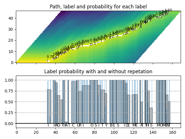
좋습니다.
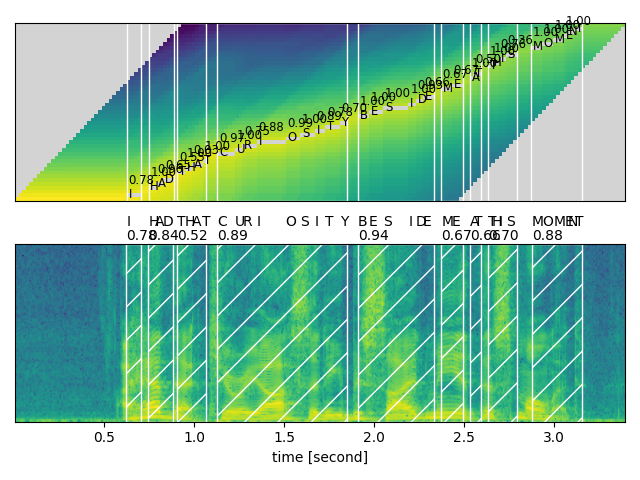
여러 분할을 단어로 병합#
지금 단어로 병합해봅시다. wav2vec2 모델은 '|' 을 단어 경계로 사용합니다.
그래서 '|' 이 등장할 때마다 분할을 병합합니다.
그러고 나서 최종적으로 원본 오디오를 분할된 오디오로 분할하고 이를 들어 분할이 옳게 되었는지 확인합니다.
# 단어 병합
def merge_words(segments, separator="|"):
    words = []
    i1, i2 = 0, 0
    while i1 < len(segments):
        if i2 >= len(segments) or segments[i2].label == separator:
            if i1 != i2:
                segs = segments[i1:i2]
                word = "".join([seg.label for seg in segs])
                score = sum(seg.score * seg.length for seg in segs) / sum(seg.length for seg in segs)
                words.append(Segment(word, segments[i1].start, segments[i2 - 1].end, score))
            i1 = i2 + 1
            i2 = i1
        else:
            i2 += 1
    return words


word_segments = merge_words(segments)
for word in word_segments:
    print(word)
I       (0.78): [   31,    35)
HAD     (0.84): [   37,    44)
THAT    (0.52): [   45,    53)
CURIOSITY       (0.89): [   56,    92)
BESIDE  (0.94): [   95,   116)
ME      (0.67): [  118,   124)
AT      (0.66): [  126,   129)
THIS    (0.70): [  131,   139)
MOMENT  (0.88): [  143,   157)
시각화#
def plot_alignments(trellis, segments, word_segments, waveform, sample_rate=bundle.sample_rate):
    trellis_with_path = trellis.clone()
    for i, seg in enumerate(segments):
        if seg.label != "|":
            trellis_with_path[seg.start : seg.end, i] = float("nan")

    fig, [ax1, ax2] = plt.subplots(2, 1)

    ax1.imshow(trellis_with_path.T, origin="lower", aspect="auto")
    ax1.set_facecolor("lightgray")
    ax1.set_xticks([])
    ax1.set_yticks([])

    for word in word_segments:
        ax1.axvspan(word.start - 0.5, word.end - 0.5, edgecolor="white", facecolor="none")

    for i, seg in enumerate(segments):
        if seg.label != "|":
            ax1.annotate(seg.label, (seg.start, i - 0.7), size="small")
            ax1.annotate(f"{seg.score:.2f}", (seg.start, i + 3), size="small")

    # 원본 waveform
    ratio = waveform.size(0) / sample_rate / trellis.size(0)
    ax2.specgram(waveform, Fs=sample_rate)
    for word in word_segments:
        x0 = ratio * word.start
        x1 = ratio * word.end
        ax2.axvspan(x0, x1, facecolor="none", edgecolor="white", hatch="/")
        ax2.annotate(f"{word.score:.2f}", (x0, sample_rate * 0.51), annotation_clip=False)

    for seg in segments:
        if seg.label != "|":
            ax2.annotate(seg.label, (seg.start * ratio, sample_rate * 0.55), annotation_clip=False)
    ax2.set_xlabel("time [second]")
    ax2.set_yticks([])
    fig.tight_layout()


plot_alignments(
    trellis,
    segments,
    word_segments,
    waveform[0],
)
오디오 샘플#
def display_segment(i):
    ratio = waveform.size(1) / trellis.size(0)
    word = word_segments[i]
    x0 = int(ratio * word.start)
    x1 = int(ratio * word.end)
    print(f"{word.label} ({word.score:.2f}): {x0 / bundle.sample_rate:.3f} - {x1 / bundle.sample_rate:.3f} sec")
    segment = waveform[:, x0:x1]
    return IPython.display.Audio(segment.numpy(), rate=bundle.sample_rate)
# 각 분할에 해당하는 오디오 생성
print(transcript)
IPython.display.Audio(SPEECH_FILE)
|I|HAD|THAT|CURIOSITY|BESIDE|ME|AT|THIS|MOMENT|
display_segment(0)
I (0.78): 0.624 - 0.704 sec
display_segment(1)
HAD (0.84): 0.744 - 0.885 sec
display_segment(2)
THAT (0.52): 0.905 - 1.066 sec
display_segment(3)
CURIOSITY (0.89): 1.127 - 1.851 sec
display_segment(4)
BESIDE (0.94): 1.911 - 2.334 sec
display_segment(5)
ME (0.67): 2.374 - 2.495 sec
display_segment(6)
AT (0.66): 2.535 - 2.595 sec
display_segment(7)
THIS (0.70): 2.635 - 2.796 sec
display_segment(8)
MOMENT (0.88): 2.877 - 3.159 sec
결론#
이번 튜토리얼에서, torchaudio의 wav2vec2 모델을 사용하여 강제 정렬을 위한 CTC 분할을 수행하는 방법을 살펴보았습니다.
Total running time of the script: (0 minutes 11.393 seconds)
