


참고
Go to the end to download the full example code.
Introduction || Tensors || Autograd || Building Models || TensorBoard Support || Training Models || Model Understanding
PyTorch TensorBoard 지원#
번역: 박정은
아래 영상이나 youtube를 참고하세요.
시작하기에 앞서#
이 튜토리얼을 실행하기 위해서 PyTorch, TorchVision, Matplotlib 그리고 TensorBoard를 설치해야 합니다.
conda 사용 시:
conda install pytorch torchvision -c pytorch
conda install matplotlib tensorboard
pip 사용 시:
pip install torch torchvision matplotlib tensorboard
한번 의존성이 있는 모듈을 설치하고 나서, 설치한 환경에서 이 notebook을 다시 시작합니다.
개요#
이 notebook에서는 변형된 LeNet-5를 Fashion-MNIST 데이터셋으로 학습시킬 것입니다. Fashion-MNIST는 의복의 종류를 나타내는 10개의 클래스 레이블을 포함하는 다양한 의류의 타일 이미지 세트입니다.
# PyTorch 모델과 훈련 필수 요소
import torch
import torch.nn as nn
import torch.nn.functional as F
import torch.optim as optim

# 이미지 데이터셋과 이미지 조작
import torchvision
import torchvision.transforms as transforms

# 이미지 시각화
import matplotlib.pyplot as plt
import numpy as np

# PyTorch TensorBoard 지원
from torch.utils.tensorboard import SummaryWriter

# 만약 Google Colab처럼 TensorFlow가 설치된 환경을 사용 중이라면
# 아래의 코드를 주석 해제하여
# TensorBoard 디렉터리에 임베딩을 저장할 때의 버그를 방지하세요.

# import tensorflow as tf
# import tensorboard as tb
# tf.io.gfile = tb.compat.tensorflow_stub.io.gfile
TensorBoard에서 이미지 나타내기#
먼저, 데이터셋에서 TensorBoard로 샘플 이미지를 추가합니다:
# 데이터셋을 모아서 사용 가능하도록 준비하기
transform = transforms.Compose(
[transforms.ToTensor(),
transforms.Normalize((0.5,), (0.5,))])
# 훈련과 검증으로 분할하여 각각 ./data에 저장하기
training_set = torchvision.datasets.FashionMNIST('./data',
download=True,
train=True,
transform=transform)
validation_set = torchvision.datasets.FashionMNIST('./data',
download=True,
train=False,
transform=transform)
training_loader = torch.utils.data.DataLoader(training_set,
batch_size=4,
shuffle=True,
num_workers=2)
validation_loader = torch.utils.data.DataLoader(validation_set,
batch_size=4,
shuffle=False,
num_workers=2)
# 클래스 레이블
classes = ('T-shirt/top', 'Trouser', 'Pullover', 'Dress', 'Coat',
'Sandal', 'Shirt', 'Sneaker', 'Bag', 'Ankle Boot')
# 인라인 이미지 시각화를 위한 함수
def matplotlib_imshow(img, one_channel=False):
if one_channel:
img = img.mean(dim=0)
img = img / 2 + 0.5 # 비정규화(unnormalize)
npimg = img.numpy()
if one_channel:
plt.imshow(npimg, cmap="Greys")
else:
plt.imshow(np.transpose(npimg, (1, 2, 0)))
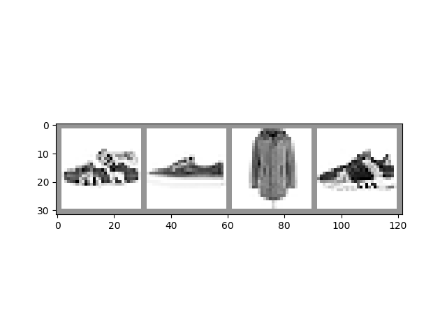
# 4개의 이미지로부터 배치 하나를 추출하기
dataiter = iter(training_loader)
images, labels = next(dataiter)
# 이미지를 나타내기 위한 격자 생성
img_grid = torchvision.utils.make_grid(images)
matplotlib_imshow(img_grid, one_channel=True)
  0%|          | 0.00/26.4M [00:00<?, ?B/s]
  0%|          | 32.8k/26.4M [00:00<03:28, 126kB/s]
  0%|          | 65.5k/26.4M [00:00<03:29, 126kB/s]
  0%|          | 98.3k/26.4M [00:00<03:29, 125kB/s]
  1%|          | 229k/26.4M [00:01<01:35, 274kB/s]
  2%|▏         | 459k/26.4M [00:01<00:52, 491kB/s]
  3%|▎         | 918k/26.4M [00:01<00:27, 922kB/s]
  7%|▋         | 1.84M/26.4M [00:01<00:13, 1.77MB/s]
 14%|█▍        | 3.67M/26.4M [00:02<00:06, 3.44MB/s]
 27%|██▋       | 7.01M/26.4M [00:02<00:03, 6.01MB/s]
 29%|██▉       | 7.60M/26.4M [00:02<00:03, 5.16MB/s]
 42%|████▏     | 11.0M/26.4M [00:02<00:02, 7.61MB/s]
 49%|████▉     | 12.9M/26.4M [00:03<00:01, 6.99MB/s]
 59%|█████▉    | 15.6M/26.4M [00:03<00:01, 7.99MB/s]
 69%|██████▉   | 18.2M/26.4M [00:03<00:01, 8.21MB/s]
 72%|███████▏  | 19.0M/26.4M [00:03<00:00, 7.56MB/s]
 82%|████████▏ | 21.7M/26.4M [00:04<00:00, 10.3MB/s]
 87%|████████▋ | 23.0M/26.4M [00:04<00:00, 9.65MB/s]
 91%|█████████▏| 24.2M/26.4M [00:04<00:00, 10.0MB/s]
 96%|█████████▌| 25.3M/26.4M [00:04<00:00, 9.13MB/s]
100%|██████████| 26.4M/26.4M [00:04<00:00, 5.80MB/s]

  0%|          | 0.00/29.5k [00:00<?, ?B/s]
100%|██████████| 29.5k/29.5k [00:00<00:00, 113kB/s]
100%|██████████| 29.5k/29.5k [00:00<00:00, 113kB/s]

  0%|          | 0.00/4.42M [00:00<?, ?B/s]
  1%|          | 32.8k/4.42M [00:00<00:35, 124kB/s]
  1%|▏         | 65.5k/4.42M [00:00<00:35, 124kB/s]
  3%|▎         | 131k/4.42M [00:00<00:23, 181kB/s]
  4%|▍         | 197k/4.42M [00:01<00:20, 208kB/s]
 10%|▉         | 426k/4.42M [00:01<00:08, 446kB/s]
 19%|█▊        | 819k/4.42M [00:01<00:04, 801kB/s]
 37%|███▋      | 1.64M/4.42M [00:01<00:01, 1.55MB/s]
 74%|███████▍  | 3.28M/4.42M [00:02<00:00, 3.03MB/s]
100%|██████████| 4.42M/4.42M [00:02<00:00, 2.08MB/s]

  0%|          | 0.00/5.15k [00:00<?, ?B/s]
100%|██████████| 5.15k/5.15k [00:00<00:00, 18.4MB/s]
위에서 TorchVision과 Matplotlib을 사용하여
입력 데이터의 미니 배치를 시각적으로 배열한 격자를 만들었습니다. 아래에서는 TensorBoard에서 사용될
이미지를 기록하기 위해 SummaryWriter 의 add_image() 를 호출하고,
또한 flush() 를 호출하여 이미지가 즉시 디스크에 기록되도록 합니다.
# log_dir 인수 기본값은 "runs"입니다 - 하지만 구체적으로 정하는 것이 좋습니다.
# 위에서 torch.utils.tensorboard.SummaryWriter를 가져왔습니다.
writer = SummaryWriter('runs/fashion_mnist_experiment_1')

# TensorBoard 로그 디렉터리에 이미지 데이터 쓰기(write)
writer.add_image('Four Fashion-MNIST Images', img_grid)
writer.flush()

# 눈으로 보기 위해서는 커맨드 라인에서 TensorBoard를 시작하세요:
#   tensorboard --logdir=runs
# ...그런 다음 브라우저에서 http://localhost:6006/ 를 열어보세요.
만약 TensorBoard를 커맨드 라인에서 구동시켜 그것을 새 브라우저 탭(보통 localhost:6006)에서 열었다면, IMAGES 탭에서 이미지 격자를 확인할 수 있을 것입니다.
훈련 시각화를 위한 스칼라 그래프 그리기#
TensorBoard는 훈련 진행 과정과 효과를 추적하기에 유용합니다. 아래에서 훈련 루프를 실행하고 몇몇 지표를 추적하며 TensorBoard에서 사용할 데이터를 저장할 것입니다.
이미지 타일을 분류할 모델과 옵티마이저 그리고 훈련의 손실 함수를 정의해 봅시다:
class Net(nn.Module):
    def __init__(self):
        super(Net, self).__init__()
        self.conv1 = nn.Conv2d(1, 6, 5)
        self.pool = nn.MaxPool2d(2, 2)
        self.conv2 = nn.Conv2d(6, 16, 5)
        self.fc1 = nn.Linear(16 * 4 * 4, 120)
        self.fc2 = nn.Linear(120, 84)
        self.fc3 = nn.Linear(84, 10)

    def forward(self, x):
        x = self.pool(F.relu(self.conv1(x)))
        x = self.pool(F.relu(self.conv2(x)))
        x = x.view(-1, 16 * 4 * 4)
        x = F.relu(self.fc1(x))
        x = F.relu(self.fc2(x))
        x = self.fc3(x)
        return x


net = Net()
criterion = nn.CrossEntropyLoss()
optimizer = optim.SGD(net.parameters(), lr=0.001, momentum=0.9)
이제 단일 에폭을 훈련하고, 매 1000 배치마다 훈련 셋과 검증 셋의 손실을 평가해 봅니다:
print(len(validation_loader))
for epoch in range(1):  # 데이터 셋을 여러 번 반복(필요 시 횟수를 조정합니다.)
    running_loss = 0.0

    for i, data in enumerate(training_loader, 0):
        # 기본 훈련 루프
        inputs, labels = data
        optimizer.zero_grad()
        outputs = net(inputs)
        loss = criterion(outputs, labels)
        loss.backward()
        optimizer.step()

        running_loss += loss.item()
        if i % 1000 == 999:    # 매 1000 미니 배치마다...
            print('Batch {}'.format(i + 1))
            # 검증 셋과 비교
            running_vloss = 0.0

            # 평가 모드에서는 일부 모델의 특정 작업을 생략할 수 있습니다 예시: 드롭아웃 레이어
            net.train(False) # 평가 모드로 전환, 예시: 정규화(regularisation) 끄기
            for j, vdata in enumerate(validation_loader, 0):
                vinputs, vlabels = vdata
                voutputs = net(vinputs)
                vloss = criterion(voutputs, vlabels)
                running_vloss += vloss.item()
            net.train(True) # 훈련 모드로 돌아가기, 예시: 정규화 켜기

            avg_loss = running_loss / 1000
            avg_vloss = running_vloss / len(validation_loader)

            # 배치별 평균 실행 손실을 기록
            writer.add_scalars('Training vs. Validation Loss',
                            { 'Training' : avg_loss, 'Validation' : avg_vloss },
                            epoch * len(training_loader) + i)

            running_loss = 0.0
print('Finished Training')

writer.flush()
2500
Batch 1000
Batch 2000
Batch 3000
Batch 4000
Batch 5000
Batch 6000
Batch 7000
Batch 8000
Batch 9000
Batch 10000
Batch 11000
Batch 12000
Batch 13000
Batch 14000
Batch 15000
Finished Training
열린 TensorBoard로 전환하여 SCALARS탭을 살펴보세요.
모델 시각화하기#
TensorBoard는 모델 내 데이터 흐름을 검사하는 데에도 유용합니다.
이를 위해, 모델과 샘플 입력을 이용해 add_graph() 메소드를
호출합니다:
# 다시, 이미지의 미니 배치 하나를 가져옵니다.
dataiter = iter(training_loader)
images, labels = next(dataiter)

# add_graph()는 샘플 입력이 모델을 통과하는 과정을 추적하고,
# 이를 그래프로 시각화합니다.
writer.add_graph(net, images)
writer.flush()
TensorBoard로 전환하면, GRAPHS 탭이 보일 것입니다. “NET” 노드를 더블 클릭하여 모델 내 계층과 데이터 흐름을 확인하세요.
임베딩으로 데이터셋 시각화하기#
우리가 사용하는 28x28 이미지 타일은 784차원의
벡터(28 * 28 = 784)가 될 수 있습니다. 더 낮은 차원으로 투영하는 쪽이
유리할 수 있습니다. add_embedding() 메소드는
가장 분산이 높은 세 차원으로 데이터 세트를 투영하고,
상호작용 가능한 3D 차트로 시각화해 줄 것입니다. add_embedding()
메소드는 가장 높은 분산을 가진 세 차원에 자동적으로
투영하여 이를 수행합니다.
아래에서 데이터 샘플을 가져와 임베딩을 생성할 것입니다:
# 데이터의 랜덤 부분집합과 대응하는 레이블을 선택
def select_n_random(data, labels, n=100):
    assert len(data) == len(labels)

    perm = torch.randperm(len(data))
    return data[perm][:n], labels[perm][:n]

# 데이터의 랜덤 부분집합 추출
images, labels = select_n_random(training_set.data, training_set.targets)

# 각 이미지별 클래스 레이블 얻기(get)
class_labels = [classes[label] for label in labels]

# 로그 임베딩
features = images.view(-1, 28 * 28)
writer.add_embedding(features,
                    metadata=class_labels,
                    label_img=images.unsqueeze(1))
writer.flush()
writer.close()
이제 TensorBoard로 전환하여 PROJECTOR 탭을 선택하면, 3D로 표현된 투영이 보일 것입니다. 그 모델을 회전하거나 확대할 수 있습니다. 크거나 작은 규모(scale)로 그것을 살펴보며, 투영된 데이터와 레이블의 클러스터링에서 패턴을 발견할 수 있는지 보세요.
가시성을 높이려면, 다음을 권장합니다:
좌측에 있는 “Color by” 드롭다운에서 “label”을 선택하세요.
상단에 있는 야간 모드 아이콘을 전환(toggle)하여 밝은 색상 이미지를 어두운 배경 위에 배치할 수 있습니다.
기타 자료#
더 알고 싶다면 여기를 참조하세요:
torch.utils.tensorboard.SummaryWriter에 대한 PyTorch 문서
PyTorch.org Tutorials에 있는 Tensorboard 튜토리얼 콘텐츠
TensorBoard에 대한 보다 더 자세한 내용은 TensorBoard 문서를 참고하세요.
Total running time of the script: (9 minutes 37.699 seconds)
