


참고
Go to the end to download the full example code.
Introduction || Tensors || Autograd || Building Models || TensorBoard Support || Training Models || Model Understanding
Training with PyTorch#
Follow along with the video below or on youtube.
Introduction#
In past videos, we’ve discussed and demonstrated:
Building models with the neural network layers and functions of the torch.nn module
The mechanics of automated gradient computation, which is central to gradient-based model training
Using TensorBoard to visualize training progress and other activities
In this video, we’ll be adding some new tools to your inventory:
We’ll get familiar with the dataset and dataloader abstractions, and how they ease the process of feeding data to your model during a training loop
We’ll discuss specific loss functions and when to use them
We’ll look at PyTorch optimizers, which implement algorithms to adjust model weights based on the outcome of a loss function
Finally, we’ll pull all of these together and see a full PyTorch training loop in action.
Dataset and DataLoader#
The Dataset and DataLoader classes encapsulate the process of
pulling your data from storage and exposing it to your training loop in
batches.
The Dataset is responsible for accessing and processing single
instances of data.
The DataLoader pulls instances of data from the Dataset (either
automatically or with a sampler that you define), collects them in
batches, and returns them for consumption by your training loop. The
DataLoader works with all kinds of datasets, regardless of the type
of data they contain.
For this tutorial, we’ll be using the Fashion-MNIST dataset provided by
TorchVision. We use torchvision.transforms.Normalize() to
zero-center and normalize the distribution of the image tile content,
and download both training and validation data splits.
import torch
import torchvision
import torchvision.transforms as transforms

# PyTorch TensorBoard support
from torch.utils.tensorboard import SummaryWriter
from datetime import datetime


transform = transforms.Compose(
    [transforms.ToTensor(),
    transforms.Normalize((0.5,), (0.5,))])

# Create datasets for training & validation, download if necessary
training_set = torchvision.datasets.FashionMNIST('./data', train=True, transform=transform, download=True)
validation_set = torchvision.datasets.FashionMNIST('./data', train=False, transform=transform, download=True)

# Create data loaders for our datasets; shuffle for training, not for validation
training_loader = torch.utils.data.DataLoader(training_set, batch_size=4, shuffle=True)
validation_loader = torch.utils.data.DataLoader(validation_set, batch_size=4, shuffle=False)

# Class labels
classes = ('T-shirt/top', 'Trouser', 'Pullover', 'Dress', 'Coat',
        'Sandal', 'Shirt', 'Sneaker', 'Bag', 'Ankle Boot')

# Report split sizes
print('Training set has {} instances'.format(len(training_set)))
print('Validation set has {} instances'.format(len(validation_set)))
Training set has 60000 instances
Validation set has 10000 instances
As always, let’s visualize the data as a sanity check:
import matplotlib.pyplot as plt
import numpy as np

# Helper function for inline image display
def matplotlib_imshow(img, one_channel=False):
    if one_channel:
        img = img.mean(dim=0)
    img = img / 2 + 0.5     # unnormalize
    npimg = img.numpy()
    if one_channel:
        plt.imshow(npimg, cmap="Greys")
    else:
        plt.imshow(np.transpose(npimg, (1, 2, 0)))

dataiter = iter(training_loader)
images, labels = next(dataiter)

# Create a grid from the images and show them
img_grid = torchvision.utils.make_grid(images)
matplotlib_imshow(img_grid, one_channel=True)
print('  '.join(classes[labels[j]] for j in range(4)))
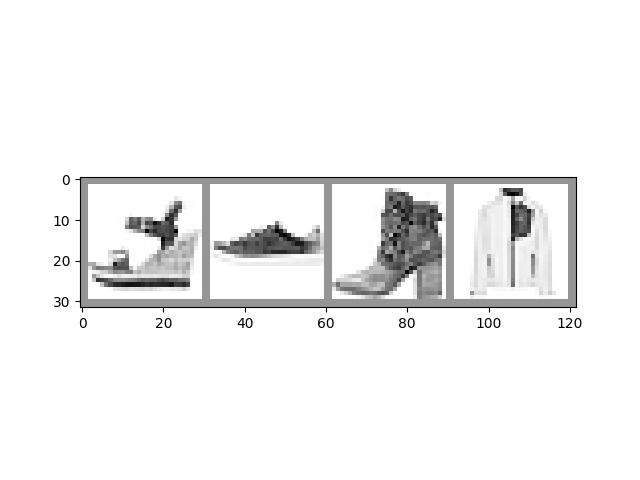
Shirt T-shirt/top Bag Shirt
The Model#
The model we’ll use in this example is a variant of LeNet-5 - it should be familiar if you’ve watched the previous videos in this series.
import torch.nn as nn
import torch.nn.functional as F

# PyTorch models inherit from torch.nn.Module
class GarmentClassifier(nn.Module):
    def __init__(self):
        super(GarmentClassifier, self).__init__()
        self.conv1 = nn.Conv2d(1, 6, 5)
        self.pool = nn.MaxPool2d(2, 2)
        self.conv2 = nn.Conv2d(6, 16, 5)
        self.fc1 = nn.Linear(16 * 4 * 4, 120)
        self.fc2 = nn.Linear(120, 84)
        self.fc3 = nn.Linear(84, 10)

    def forward(self, x):
        x = self.pool(F.relu(self.conv1(x)))
        x = self.pool(F.relu(self.conv2(x)))
        x = x.view(-1, 16 * 4 * 4)
        x = F.relu(self.fc1(x))
        x = F.relu(self.fc2(x))
        x = self.fc3(x)
        return x


model = GarmentClassifier()
Loss Function#
For this example, we’ll be using a cross-entropy loss. For demonstration purposes, we’ll create batches of dummy output and label values, run them through the loss function, and examine the result.
loss_fn = torch.nn.CrossEntropyLoss()

# NB: Loss functions expect data in batches, so we're creating batches of 4
# Represents the model's confidence in each of the 10 classes for a given input
dummy_outputs = torch.rand(4, 10)
# Represents the correct class among the 10 being tested
dummy_labels = torch.tensor([1, 5, 3, 7])

print(dummy_outputs)
print(dummy_labels)

loss = loss_fn(dummy_outputs, dummy_labels)
print('Total loss for this batch: {}'.format(loss.item()))
tensor([[0.2133, 0.5840, 0.9250, 0.3898, 0.5711, 0.1149, 0.1957, 0.0159, 0.6406,
         0.4990],
        [0.1759, 0.6216, 0.7666, 0.5881, 0.6539, 0.7655, 0.1511, 0.2223, 0.6214,
         0.7261],
        [0.3302, 0.4371, 0.1898, 0.6498, 0.1435, 0.4840, 0.1881, 0.1893, 0.3586,
         0.5927],
        [0.5817, 0.9643, 0.4310, 0.1324, 0.6099, 0.8136, 0.8432, 0.4990, 0.7913,
         0.6154]])
tensor([1, 5, 3, 7])
Total loss for this batch: 2.1856586933135986
Optimizer#
For this example, we’ll be using simple stochastic gradient descent with momentum.
It can be instructive to try some variations on this optimization scheme:
Learning rate determines the size of the steps the optimizer takes. What does a different learning rate do to the your training results, in terms of accuracy and convergence time?
Momentum nudges the optimizer in the direction of strongest gradient over multiple steps. What does changing this value do to your results?
Try some different optimization algorithms, such as averaged SGD, Adagrad, or Adam. How do your results differ?
# Optimizers specified in the torch.optim package
optimizer = torch.optim.SGD(model.parameters(), lr=0.001, momentum=0.9)
The Training Loop#
Below, we have a function that performs one training epoch. It enumerates data from the DataLoader, and on each pass of the loop does the following:
Gets a batch of training data from the DataLoader
Zeros the optimizer’s gradients
Performs an inference - that is, gets predictions from the model for an input batch
Calculates the loss for that set of predictions vs. the labels on the dataset
Calculates the backward gradients over the learning weights
Tells the optimizer to perform one learning step - that is, adjust the model’s learning weights based on the observed gradients for this batch, according to the optimization algorithm we chose
It reports on the loss for every 1000 batches.
Finally, it reports the average per-batch loss for the last 1000 batches, for comparison with a validation run
def train_one_epoch(epoch_index, tb_writer):
    running_loss = 0.
    last_loss = 0.

    # Here, we use enumerate(training_loader) instead of
    # iter(training_loader) so that we can track the batch
    # index and do some intra-epoch reporting
    for i, data in enumerate(training_loader):
        # Every data instance is an input + label pair
        inputs, labels = data

        # Zero your gradients for every batch!
        optimizer.zero_grad()

        # Make predictions for this batch
        outputs = model(inputs)

        # Compute the loss and its gradients
        loss = loss_fn(outputs, labels)
        loss.backward()

        # Adjust learning weights
        optimizer.step()

        # Gather data and report
        running_loss += loss.item()
        if i % 1000 == 999:
            last_loss = running_loss / 1000 # loss per batch
            print('  batch {} loss: {}'.format(i + 1, last_loss))
            tb_x = epoch_index * len(training_loader) + i + 1
            tb_writer.add_scalar('Loss/train', last_loss, tb_x)
            running_loss = 0.

    return last_loss
Per-Epoch Activity#
There are a couple of things we’ll want to do once per epoch:
Perform validation by checking our relative loss on a set of data that was not used for training, and report this
Save a copy of the model
Here, we’ll do our reporting in TensorBoard. This will require going to the command line to start TensorBoard, and opening it in another browser tab.
# Initializing in a separate cell so we can easily add more epochs to the same run
timestamp = datetime.now().strftime('%Y%m%d_%H%M%S')
writer = SummaryWriter('runs/fashion_trainer_{}'.format(timestamp))
epoch_number = 0

EPOCHS = 5

best_vloss = 1_000_000.

for epoch in range(EPOCHS):
    print('EPOCH {}:'.format(epoch_number + 1))

    # Make sure gradient tracking is on, and do a pass over the data
    model.train(True)
    avg_loss = train_one_epoch(epoch_number, writer)


    running_vloss = 0.0
    # Set the model to evaluation mode, disabling dropout and using population
    # statistics for batch normalization.
    model.eval()

    # Disable gradient computation and reduce memory consumption.
    with torch.no_grad():
        for i, vdata in enumerate(validation_loader):
            vinputs, vlabels = vdata
            voutputs = model(vinputs)
            vloss = loss_fn(voutputs, vlabels)
            running_vloss += vloss

    avg_vloss = running_vloss / (i + 1)
    print('LOSS train {} valid {}'.format(avg_loss, avg_vloss))

    # Log the running loss averaged per batch
    # for both training and validation
    writer.add_scalars('Training vs. Validation Loss',
                    { 'Training' : avg_loss, 'Validation' : avg_vloss },
                    epoch_number + 1)
    writer.flush()

    # Track best performance, and save the model's state
    if avg_vloss < best_vloss:
        best_vloss = avg_vloss
        model_path = 'model_{}_{}'.format(timestamp, epoch_number)
        torch.save(model.state_dict(), model_path)

    epoch_number += 1
EPOCH 1:
  batch 1000 loss: 1.7172835692167283
  batch 2000 loss: 0.848677432352677
  batch 3000 loss: 0.7013446503840387
  batch 4000 loss: 0.6292305398017634
  batch 5000 loss: 0.5705106372283771
  batch 6000 loss: 0.530786006947048
  batch 7000 loss: 0.5168804385215044
  batch 8000 loss: 0.5366029786192812
  batch 9000 loss: 0.4827208117973059
  batch 10000 loss: 0.4458405884082895
  batch 11000 loss: 0.43226282635168173
  batch 12000 loss: 0.4351422864545602
  batch 13000 loss: 0.416676636031596
  batch 14000 loss: 0.41562795037950856
  batch 15000 loss: 0.41219041802675926
LOSS train 0.41219041802675926 valid 0.40465718507766724
EPOCH 2:
  batch 1000 loss: 0.39023975565540603
  batch 2000 loss: 0.3699741753226263
  batch 3000 loss: 0.3782766498834244
  batch 4000 loss: 0.38281650762917707
  batch 5000 loss: 0.3781999181426363
  batch 6000 loss: 0.3806056835514319
  batch 7000 loss: 0.35880676115385723
  batch 8000 loss: 0.36294173052784756
  batch 9000 loss: 0.35123865842125085
  batch 10000 loss: 0.3433105904458789
  batch 11000 loss: 0.35292539940564893
  batch 12000 loss: 0.34155431485932786
  batch 13000 loss: 0.3565417002681934
  batch 14000 loss: 0.3470489102199499
  batch 15000 loss: 0.3324835271326592
LOSS train 0.3324835271326592 valid 0.35021084547042847
EPOCH 3:
  batch 1000 loss: 0.3099278601160622
  batch 2000 loss: 0.3134169123527099
  batch 3000 loss: 0.3101419919889304
  batch 4000 loss: 0.32413815653455097
  batch 5000 loss: 0.3149802439641207
  batch 6000 loss: 0.32601341716657045
  batch 7000 loss: 0.3057375025972378
  batch 8000 loss: 0.32355299448716685
  batch 9000 loss: 0.3270067947786447
  batch 10000 loss: 0.3370232685001101
  batch 11000 loss: 0.28910923016078593
  batch 12000 loss: 0.31505058472105885
  batch 13000 loss: 0.3088230035615416
  batch 14000 loss: 0.31752997355678236
  batch 15000 loss: 0.3121288968419831
LOSS train 0.3121288968419831 valid 0.32703542709350586
EPOCH 4:
  batch 1000 loss: 0.2707901962498436
  batch 2000 loss: 0.29014508830209523
  batch 3000 loss: 0.31546937639992395
  batch 4000 loss: 0.3032910483292362
  batch 5000 loss: 0.2900829899934761
  batch 6000 loss: 0.290307943903812
  batch 7000 loss: 0.2982047825271729
  batch 8000 loss: 0.30285163901646595
  batch 9000 loss: 0.2911962075142292
  batch 10000 loss: 0.28399802248621925
  batch 11000 loss: 0.2881571567760839
  batch 12000 loss: 0.27252229429695535
  batch 13000 loss: 0.2964596547502624
  batch 14000 loss: 0.27943266273821793
  batch 15000 loss: 0.2938154865120814
LOSS train 0.2938154865120814 valid 0.31321677565574646
EPOCH 5:
  batch 1000 loss: 0.27343099248513864
  batch 2000 loss: 0.27009573868704867
  batch 3000 loss: 0.2775436939162901
  batch 4000 loss: 0.27996335977715536
  batch 5000 loss: 0.2783755845226824
  batch 6000 loss: 0.25646028433018364
  batch 7000 loss: 0.27602541703587485
  batch 8000 loss: 0.2678100048684637
  batch 9000 loss: 0.2718898843228526
  batch 10000 loss: 0.25534316919115735
  batch 11000 loss: 0.2761891596711648
  batch 12000 loss: 0.26931544719509837
  batch 13000 loss: 0.2829810179315159
  batch 14000 loss: 0.2646401177785037
  batch 15000 loss: 0.28811035650204575
LOSS train 0.28811035650204575 valid 0.2991027534008026
To load a saved version of the model:
saved_model = GarmentClassifier()
saved_model.load_state_dict(torch.load(PATH))
Once you’ve loaded the model, it’s ready for whatever you need it for - more training, inference, or analysis.
Note that if your model has constructor parameters that affect model structure, you’ll need to provide them and configure the model identically to the state in which it was saved.
Other Resources#
Docs on the data utilities, including Dataset and DataLoader, at pytorch.org
A note on the use of pinned memory for GPU training
Documentation on the datasets available in TorchVision, TorchText, and TorchAudio
Documentation on the loss functions available in PyTorch
Documentation on the torch.optim package, which includes optimizers and related tools, such as learning rate scheduling
A detailed tutorial on saving and loading models
The Tutorials section of pytorch.org contains tutorials on a broad variety of training tasks, including classification in different domains, generative adversarial networks, reinforcement learning, and more
Total running time of the script: (22 minutes 40.382 seconds)
