(프로토타입) 반정형적 (2:4) 희소성(semi-structured (2:4) sparsity)을 이용한 BERT 가속화하기

저자: Jesse Cai 번역: Dabin Kang

다른 형태의 희소성처럼, 반정형적 희소성(semi-structured sparsity)**은 메모리 오버헤드와 지연 시간을 줄이기 위한 모델 최적화 기법으로, 일부 모델 정확도를 희생하면서 이점을 얻습니다. 반정형적 희소성은 **fine-grained structured sparsity 또는 **2:4 structured sparsity**라고도 불립니다.

반정형적 희소성은 2n개의 요소 중 n개의 요소가 제거되는 독특한 희소성 패턴에서 그 이름을 따왔습니다. 가장 일반적으로 n=2가 적용되므로 2:4 희소성이라고 불립니다. 반정형적 희소성은 특히 GPU에서 효율적으로 가속화될 수 있고, 다른 희소성 패턴보다 모델의 정확도를 덜 저하시키기 때문에 흥미롭습니다.

`반정형적 희소성 지원 <https://pytorch.org/docs/2.1/sparse.html#sparse-semi-structured-tensors>`_으로, PyTorch 환경에서 반정형적 희소 모델을 가지치기하고 가속화할 수 있습니다. 이 튜토리얼에서 그 과정을 설명하겠습니다.

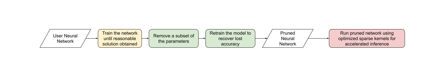
이 튜토리얼을 끝내면, 2:4 희소성으로 가지치기하고, 거의 모든 F1 손실(밀집 86.92 vs 희소 86.48)을 복구하도록 미세 조정한 BERT 질문-답변 모델이 완성됩니다. 마지막으로, 이 2:4 희소 모델을 추론 단계에서 가속화하여 1.3배의 속도 향상을 달성할 것입니다.

요구 사항

• PyTorch >= 2.1.

• 반정형적 희소성을 지원하는 NVIDIA GPU (Compute Capability 8.0+).

참고

이 튜토리얼은 반정형적 희소성 또는 일반적인 희소성에 익숙하지 않은 초보자를 위해 설계되었습니다. 기존 2:4 희소 모델이 있다면, to_sparse_semi_structured``를 사용하여 ``nn.Linear 레이어를 추론을 위해 가속화하면 간단합니다 :

import torch
from torch.sparse import to_sparse_semi_structured, SparseSemiStructuredTensor
from torch.utils.benchmark import Timer
SparseSemiStructuredTensor._FORCE_CUTLASS = True

# 2:4 희소성을 가지도록 Linear 가중치에 마스크 적용
mask = torch.Tensor([0, 0, 1, 1]).tile((3072, 2560)).cuda().bool()
linear = torch.nn.Linear(10240, 3072).half().cuda().eval()
linear.weight = torch.nn.Parameter(mask * linear.weight)

x = torch.rand(3072, 10240).half().cuda()

with torch.inference_mode():
    dense_output = linear(x)
    dense_t = Timer(stmt="linear(x)",
                    globals={"linear": linear,
                             "x": x}).blocked_autorange().median * 1e3

    # SparseSemiStructuredTensor로 가속화
    linear.weight = torch.nn.Parameter(to_sparse_semi_structured(linear.weight))

    sparse_output = linear(x)
    sparse_t = Timer(stmt="linear(x)",
                    globals={"linear": linear,
                             "x": x}).blocked_autorange().median * 1e3

    # 희소성과 밀집 행렬 곱셈(dense matmul)은 수치적으로 동일
    assert torch.allclose(sparse_output, dense_output, atol=1e-3)
    print(f"Dense: {dense_t:.3f}ms Sparse: {sparse_t:.3f}ms | Speedup: {(dense_t / sparse_t):.3f}x")

A100 80GB에서의 결과 : Dense: 0.870ms Sparse: 0.630ms | Speedup: 1.382x

반정형적 희소성이 해결하는 문제는 무엇인가?

희소성의 일반적인 동기는 간단합니다: 네트워크에 0이 있는 경우 해당 매개변수를 저장하거나 계산하지 않도록 할 수 있습니다. 하지만 희소성의 구체적인 내용은 까다롭습니다. 매개변수를 0으로 만들면 별도의 과정 없이는 모델의 지연 시간이나 메모리 오버헤드에 영향을 미치지 않습니다.

이는 밀집 tensor에 여전히 가지치기된(제로) 요소가 포함되어 있어, 밀집 행렬 곱셈 커널이 여전히 이러한 요소를 계산하기 때문입니다. 성능 향상을 얻으려면, 가지치기된 요소 계산을 건너뛰는 희소 커널로 밀집 커널을 교체해야 합니다.

이를 위해 이러한 커널은 가지치기된 요소를 저장하지 않고 지정된 요소를 압축된 형식으로 저장하는 희소 행렬에서 작동합니다.

반정형적 희소성에서는 원래 매개변수의 정확히 절반을 압축된 메타데이터와 함께 저장하여 요소가 어떻게 배열되었는지에 대한 정보를 제공합니다.

각기 다른 장단점을 가진 여러 가지 희소성 구조들이 있습니다. 특히 2:4 반정형적 희소 레이아웃은 두 가지 이유로 흥미롭습니다: 1. 이전의 희소 형식과 달리 반정형적 희소성은 GPU에서 효율적으로 가속화되도록 설계되었습니다.

2020년, NVIDIA는 Ampere 아키텍처와 함께 반정형적 희소성을 지원하는 하드웨어를 도입했으며, CUTLASS/`cuSPARSELt <https://docs.nvidia.com/cuda/cusparselt/index.html>`_를 통해 빠른 희소 커널도 출시했습니다.

2. 동시에, 특히 더 발전된 가지치기 및 미세 조정 방법을 고려할 때, 반정형적 희소성은 다른 희소 형식에 비해 모델 정확도에 미치는 영향이 적습니다. NVIDIA는 `white paper <https://arxiv.org/abs/2104.08378>`_에서 2:4 희소성을 위한 크기 기반 가지치기와 재학습하는 단순한 패러다임을 통해 거의 동일한 모델 정확도를 얻을 수 있음을 보여주었습니다.

반정형적 희소성은 50%라는 낮은 희소성 수준에서 2배의 이론적인 속도 향상을 제공하며, 모델 정확도를 유지할 수 있을 만큼 충분히 세밀합니다.

Network	Data Set	Metric	Dense FP16	Sparse FP16
ResNet-50	ImageNet	Top-1	76.1	76.2
ResNeXt-101_32x8d	ImageNet	Top-1	79.3	79.3
Xception	ImageNet	Top-1	79.2	79.2
SSD-RN50	COCO2017	bbAP	24.8	24.8
MaskRCNN-RN50	COCO2017	bbAP	37.9	37.9
FairSeq Transformer	EN-DE WMT14	BLEU	28.2	28.5
BERT-Large	SQuAD v1.1	F1	91.9	91.9

반정형적 희소성은 워크플로우 관점에서도 추가적인 이점이 있습니다. 희소성 수준이 50%로 고정되어 있어 모델을 희소화하는 문제를 두 가지 하위 문제로 분리하기가 더 쉬워집니다:

• 정확도 - 모델의 정확도 저하를 최소화할 수 있는 2:4 희소 가중치 세트를 어떻게 찾을 수 있을까요?

• 성능 - 추론을 위해 2:4 희소 가중치를 어떻게 가속화하고 메모리 오버헤드를 줄일 수 있을까요?

\[\begin{bmatrix} 1 & 1 & 0 & 0 \\ 0 & 0 & 1 & 1 \\ 1 & 0 & 0 & 0 \\ 0 & 0 & 1 & 1 \\ \end{bmatrix} \]

이 두 문제 사이의 자연스러운 핸드오프(handoff) 포인트는 0으로 된 밀집 tensor입니다. 이 형식의 tensor를 압축하고 가속화하도록 추론을 설계했습니다. 활발한 연구분야인 만큼 많은 사용자가 맞춤형 마스킹 해결책을 고안할 것으로 예상합니다.

이제 반정형적 희소성에 대해 조금 더 배웠으니, 질문 답변 작업인 SQuAD에서 학습된 BERT 모델에 이를 적용해 봅시다.

소개 & 설정

우선 필요한 모든 패키지를 불러옵시다.

import collections
import datasets
import evaluate
import numpy as np
import torch
import torch.utils.benchmark as benchmark
from torch import nn
from torch.sparse import to_sparse_semi_structured, SparseSemiStructuredTensor
from torch.ao.pruning import WeightNormSparsifier
import transformers

# cuSPARSELt가 사용 불가능한 경우 CUTLASS 사용을 강제
SparseSemiStructuredTensor._FORCE_CUTLASS = True
torch.manual_seed(100)

또한 데이터셋과 작업에 특정한 몇 가지 함수를 직접 정의해야 합니다. 이 huggingface 코스에서 참조했습니다.

def preprocess_validation_function(examples, tokenizer):
    inputs = tokenizer(
        [q.strip() for q in examples["question"]],
        examples["context"],
        max_length=384,
        truncation="only_second",
        return_overflowing_tokens=True,
        return_offsets_mapping=True,
        padding="max_length",
    )
    sample_map = inputs.pop("overflow_to_sample_mapping")
    example_ids = []

    for i in range(len(inputs["input_ids"])):
        sample_idx = sample_map[i]
        example_ids.append(examples["id"][sample_idx])
        sequence_ids = inputs.sequence_ids(i)
        offset = inputs["offset_mapping"][i]
        inputs["offset_mapping"][i] = [
            o if sequence_ids[k] == 1 else None for k, o in enumerate(offset)
        ]

    inputs["example_id"] = example_ids
    return inputs


def preprocess_train_function(examples, tokenizer):
    inputs = tokenizer(
        [q.strip() for q in examples["question"]],
        examples["context"],
        max_length=384,
        truncation="only_second",
        return_offsets_mapping=True,
        padding="max_length",
    )

    offset_mapping = inputs["offset_mapping"]
    answers = examples["answers"]
    start_positions = []
    end_positions = []

    for i, (offset, answer) in enumerate(zip(offset_mapping, answers)):
        start_char = answer["answer_start"][0]
        end_char = start_char + len(answer["text"][0])
        sequence_ids = inputs.sequence_ids(i)

        # 문맥의 시작과 끝 찾기
        idx = 0
        while sequence_ids[idx] != 1:
            idx += 1
        context_start = idx
        while sequence_ids[idx] == 1:
            idx += 1
        context_end = idx - 1

        # 답변이 문맥 내에 완전히 포함되지 않으면 (0, 0)으로 라벨링하기
        if offset[context_start][0] > end_char or offset[context_end][1] < start_char:
            start_positions.append(0)
            end_positions.append(0)
        else:
            # 그렇지 않으면 시작 및 끝 토큰 위치로 라벨링하기
            idx = context_start
            while idx <= context_end and offset[idx][0] <= start_char:
                idx += 1
            start_positions.append(idx - 1)

            idx = context_end
            while idx >= context_start and offset[idx][1] >= end_char:
                idx -= 1
            end_positions.append(idx + 1)

    inputs["start_positions"] = start_positions
    inputs["end_positions"] = end_positions
    return inputs


def compute_metrics(start_logits, end_logits, features, examples):
    n_best = 20
    max_answer_length = 30
    metric = evaluate.load("squad")

    example_to_features = collections.defaultdict(list)
    for idx, feature in enumerate(features):
        example_to_features[feature["example_id"]].append(idx)

    predicted_answers = []
    # for example in tqdm(examples):
    for example in examples:
        example_id = example["id"]
        context = example["context"]
        answers = []

        # 해당 예제와 연관된 모든 특징 반복하기
        for feature_index in example_to_features[example_id]:
            start_logit = start_logits[feature_index]
            end_logit = end_logits[feature_index]
            offsets = features[feature_index]["offset_mapping"]

            start_indexes = np.argsort(start_logit)[-1 : -n_best - 1 : -1].tolist()
            end_indexes = np.argsort(end_logit)[-1 : -n_best - 1 : -1].tolist()
            for start_index in start_indexes:
                for end_index in end_indexes:
                    # 문맥 내에 완전히 포함되지 않은 답변 건너뛰기
                    if offsets[start_index] is None or offsets[end_index] is None:
                        continue
                    # 길이가 < 0 이거나
                    # 또는 > 최대 답변 길이(max_answer_length)인 답변 건너뛰기
                    if (
                        end_index < start_index
                        or end_index - start_index + 1 > max_answer_length
                    ):
                        continue

                    answer = {
                        "text": context[
                            offsets[start_index][0] : offsets[end_index][1]
                        ],
                        "logit_score": start_logit[start_index] + end_logit[end_index],
                    }
                    answers.append(answer)

        # 가장 높은 점수를 가진 답변 선택
        if len(answers) > 0:
            best_answer = max(answers, key=lambda x: x["logit_score"])
            predicted_answers.append(
                {"id": example_id, "prediction_text": best_answer["text"]}
            )
        else:
            predicted_answers.append({"id": example_id, "prediction_text": ""})

    theoretical_answers = [
        {"id": ex["id"], "answers": ex["answers"]} for ex in examples
    ]
    return metric.compute(predictions=predicted_answers, references=theoretical_answers)

이제 함수들을 정의했으니, 모델의 실행 시간을 측정하는 추가적인 함수가 필요합니다.

def measure_execution_time(model, batch_sizes, dataset):
    dataset_for_model = dataset.remove_columns(["example_id", "offset_mapping"])
    dataset_for_model.set_format("torch")
    model.cuda()
    batch_size_to_time_sec = {}
    for batch_size in batch_sizes:
        batch = {
            k: dataset_for_model[k][:batch_size].to(model.device)
            for k in dataset_for_model.column_names
        }

        with torch.inference_mode():
            timer = benchmark.Timer(
                stmt="model(**batch)", globals={"model": model, "batch": batch}
            )
            p50 = timer.blocked_autorange().median * 1000
        batch_size_to_time_sec[batch_size] = p50
    return batch_size_to_time_sec

모델과 토크나이저를 로드하고 데이터셋을 설정하는 것으로 시작해 봅시다.

# 모델 불러오기
model_name = "bert-base-cased"
tokenizer = transformers.AutoTokenizer.from_pretrained(model_name)
model = transformers.AutoModelForQuestionAnswering.from_pretrained(model_name)
print(f"Loading tokenizer: {model_name}")
print(f"Loading model: {model_name}")

# 학습 및 검증 데이터셋 설정
squad_dataset = datasets.load_dataset("squad")
tokenized_squad_dataset = {}
tokenized_squad_dataset["train"] = squad_dataset["train"].map(
    lambda x: preprocess_train_function(x, tokenizer), batched=True
)
tokenized_squad_dataset["validation"] = squad_dataset["validation"].map(
    lambda x: preprocess_validation_function(x, tokenizer),
    batched=True,
    remove_columns=squad_dataset["train"].column_names,
)
data_collator = transformers.DataCollatorWithPadding(tokenizer=tokenizer)

다음으로, SQuAD에 대한 모델의 간단한 기본 학습을 해봅시다. 이 작업은 주어진 질문에 대한 답변을 포함하는 문맥(Wikipedia articles)에서 텍스트의 일부를 식별하는 것입니다. 다음 코드를 실행하면 F1 점수 86.9를 얻을 수 있습니다. 이는 NVIDIA의 보고된 점수와 매우 유사하며, 차이는 BERT-base와 BERT-large 또는 미세 조정 하이퍼파라미터 때문일 가능성이 큽니다.

training_args = transformers.TrainingArguments(
    "trainer",
    num_train_epochs=1,
    lr_scheduler_type="constant",
    per_device_train_batch_size=64,
    per_device_eval_batch_size=512,
)

trainer = transformers.Trainer(
    model,
    training_args,
    train_dataset=tokenized_squad_dataset["train"],
    eval_dataset=tokenized_squad_dataset["validation"],
    data_collator=data_collator,
    tokenizer=tokenizer,
)

trainer.train()

# 평가를 위해 비교할 배치 크기
batch_sizes = [4, 16, 64, 256]
# 2:4 희소성은 fp16이 필요하므로 공정한 비교를 위해 여기서 형 변환
with torch.autocast("cuda"):
    with torch.inference_mode():
        predictions = trainer.predict(tokenized_squad_dataset["validation"])
    start_logits, end_logits = predictions.predictions
    fp16_baseline = compute_metrics(
        start_logits,
        end_logits,
        tokenized_squad_dataset["validation"],
        squad_dataset["validation"],
    )
    fp16_time = measure_execution_time(
        model,
        batch_sizes,
        tokenized_squad_dataset["validation"],
    )
print("fp16", fp16_baseline)
print("cuda_fp16 time", fp16_time)

# fp16 {'exact_match': 78.53358561967833, 'f1': 86.9280493093186}
# cuda_fp16 time {4: 10.927572380751371, 16: 19.607915310189128, 64: 73.18846387788653, 256: 286.91255673766136}

BERT를 2:4 희소성으로 가지치기

이제 기본 학습이 완료되었으니, BERT를 가지치기할 차례입니다. 가지치기 전략은 여러 가지가 있지만, 가장 일반적인 것은 **크기 기반 가지치기(magnitude pruning)**로, 가장 낮은 L1 norm으로 가중치를 제거합니다. NVIDIA는 모든 결과에서 크기 기반 가지치기를 사용했으며, 이는 일반적인 기준입니다.

이를 위해 torch.ao.pruning 패키지를 사용하여 가중치-단위 (크기) 희소화를 적용할 것입니다. 이 희소화는 모델의 가중치 tensor에 마스크 매개변수를 적용합니다. 즉, 가지치기된 가중치를 마스킹하여 제거하면서 희소성을 시뮬레이션합니다.

또한, 어떤 레이어에 희소성을 적용할지 결정해야 하는데, 이 경우에는 작업 특화 헤드 출력 레이어를 제외한 모든 nn.Linear 레이어입니다. 이는 반정형적 희소성이 `형태 제약 <https://pytorch.org/docs/2.1/sparse.html#constructing-sparse-semi-structured-tensors>`_이 있기 때문이며, 작업 특화 nn.Linear 레이어는 이러한 제약을 만족하지 못합니다.

sparsifier = WeightNormSparsifier(
    # 모든 블록에 희소성을 적용
    sparsity_level=1.0,
    # 4개 요소의 블록 형태
    sparse_block_shape=(1, 4),
    # 4 블록당 두 개의 0
    zeros_per_block=2
)

# BERT 모델에서 nn.Linear가 존재하는 경우 설정에 추가
sparse_config = [
    {"tensor_fqn": f"{fqn}.weight"}
    for fqn, module in model.named_modules()
    if isinstance(module, nn.Linear) and "layer" in fqn
]

모델을 가지치기하기 위한 첫 번째 단계는 가중치 마스킹을 위한 매개변수를 삽입하는 단계입니다. 이 단계는 준비 단계로 마무리됩니다. ``.weight``에 접근할 때마다 ``mask * weight``를 얻게 됩니다.

# 모델 준비, 학습을 위한 가짜-희소성(fake-sparsity) 매개변수 삽입
sparsifier.prepare(model, sparse_config)
print(model.bert.encoder.layer[0].output)

# BertOutput(
#   (dense): ParametrizedLinear(
#     in_features=3072, out_features=768, bias=True
#     (parametrizations): ModuleDict(
#       (weight): ParametrizationList(
#         (0-5): 6 x FakeSparsity()
#       )
#     )
#   )
#   (LayerNorm): LayerNorm((768,), eps=1e-12, elementwise_affine=True)
#   (dropout): Dropout(p=0.1, inplace=False)
# )

그 다음 가지치기 단계를 한 번 실행합니다. 모든 가지치기는 update_mask() 메소드를 구현하여 가지치기 구현 논리에 따라 마스크를 업데이트합니다. step 메소드는 희소 구성에서 지정된 가중치에 대해 이 update_mask 함수를 호출합니다.

또한, 미세 조정이나 재학습 없이 가지치기되거나 학습 없이 가지치기된 모델의 정확도 저하를 보여주기 위해 모델을 평가할 것입니다.

sparsifier.step()
with torch.autocast("cuda"):
    with torch.inference_mode():
        predictions = trainer.predict(tokenized_squad_dataset["validation"])
    pruned = compute_metrics(
        *predictions.predictions,
        tokenized_squad_dataset["validation"],
        squad_dataset["validation"],
    )
print("pruned eval metrics:", pruned)
# pruned eval metrics: {'exact_match': 40.59602649006622, 'f1': 56.51610004515979}

이 상태에서 모델을 미세 조정하여 가지치기되지 않을 요소를 업데이트하고, 정확도 손실을 더 잘 반영하도록 합니다. 만족할 만한 상태에 도달하면 ``squash_mask``를 호출하여 마스크와 가중치를 함께 융합할 수 있습니다. 이렇게 하면 매개변수가 제거되고, 2:4로 밀집된 0이 있는 모델이 남게 됩니다.

trainer.train()
sparsifier.squash_mask()
torch.set_printoptions(edgeitems=4)
print(model.bert.encoder.layer[0].intermediate.dense.weight)

# Parameter containing:
# tensor([[ 0.0000, -0.0237,  0.0000,  0.0130,  ..., -0.0462, -0.0000, 0.0000, -0.0272],
#        [ 0.0436, -0.0000, -0.0000,  0.0492,  ..., -0.0000,  0.0844,  0.0340, -0.0000],
#        [-0.0302, -0.0350,  0.0000,  0.0000,  ...,  0.0303,  0.0175, -0.0000,  0.0000],
#        [ 0.0000, -0.0000, -0.0529,  0.0327,  ...,  0.0213,  0.0000, -0.0000,  0.0735],
#        ...,
#        [ 0.0000, -0.0000, -0.0258, -0.0239,  ..., -0.0000, -0.0000,  0.0380,  0.0562],
#        [-0.0432, -0.0000,  0.0000, -0.0598,  ...,  0.0000, -0.0000,  0.0262  -0.0227],
#        [ 0.0244,  0.0921, -0.0000, -0.0000,  ..., -0.0000, -0.0784,  0.0000,  0.0761],
#        [ 0.0000,  0.0225, -0.0395, -0.0000,  ..., -0.0000,  0.0684, -0.0344, -0.0000]], device='cuda:0', requires_grad=True)

2:4 희소 모델을 추론 단계에서 가속화하기 ——–i———————————— 이제 모델이 준비되었으므로 QuickStart Guide에서처럼 추론 단계에서 가속화할 수 있습니다.

model = model.cuda().half()
# 희소성으로 가속화
for fqn, module in model.named_modules():
    if isinstance(module, nn.Linear) and "layer" in fqn:
        module.weight = nn.Parameter(to_sparse_semi_structured(module.weight))

with torch.inference_mode():
    predictions = trainer.predict(tokenized_squad_dataset["validation"])
start_logits, end_logits = predictions.predictions
metrics_sparse = compute_metrics(
    start_logits,
    end_logits,
    tokenized_squad_dataset["validation"],
    squad_dataset["validation"],
)
print("sparse eval metrics: ", metrics_sparse)
sparse_perf = measure_execution_time(
    model,
    batch_sizes,
    tokenized_squad_dataset["validation"],
)
print("sparse perf metrics: ", sparse_perf)

# sparse eval metrics:  {'exact_match': 78.43897824030275, 'f1': 86.48718950090766}
# sparse perf metrics:  {4: 12.621004460379481, 16: 15.368514601141214, 64: 58.702805917710066, 256: 244.19364519417286}

크기 기반 가지치기(magnitude pruning) 후 모델을 다시 학습하여 가지치기 후 모델에서 손실된 F1의 대부분을 복구할 수 있었습니다. 동시에 bs=16에서 1.28배의 속도 향상을 달성했습니다. 성능 개선에 적합하지 않은 형태도 있습니다. 배치 크기가 작고 계산 시간이 제한적일 때 희소 커널이 밀집 커널보다 느릴 수 있습니다.

results

Metrics	fp16	2:4 sparse	delta / speedup
Exact Match (%)	78.53	78.44	-0.09
F1 (%)	86.93	86.49	-0.44
Time (bs=4)	10.93	12.62	0.87x
Time (bs=16)	19.61	15.37	1.28x
Time (bs=64)	73.19	58.70	1.25x
Time (bs=256)	286.91	244.19	1.18x

결론

이 튜토리얼에서는 BERT를 2:4 희소성으로 가지치기하고, 2:4 희소 모델을 추론 단계에서 가속화하는 방법을 보여주었습니다. SparseSemiStructuredTensor 하위 클래스를 활용하여 fp16 기본값 대비 1.3배 속도 향상을 달성할 수 있었습니다. 또한 BERT를 미세 조정하여 손실된 F1(밀집 86.92 vs 희소 86.48)을 복구할 수 있음을 입증했습니다.