


참고
Go to the end to download the full example code.
파이프라인 병렬화로 트랜스포머 모델 학습시키기#
- Author: Pritam Damania
번역: 백선희
이 튜토리얼은 파이프라인(pipeline) 병렬화(parallelism)를 사용하여 여러 GPU에 걸친 거대한 트랜스포머(transformer) 모델을 어떻게 학습시키는지 보여줍니다. NN.TRANSFORMER 와 TORCHTEXT 로 시퀀스-투-시퀀스(SEQUENCE-TO-SEQUENCE) 모델링하기 튜토리얼의 확장판이며 파이프라인 병렬화가 어떻게 트랜스포머 모델 학습에 쓰이는지 증명하기 위해 이전 튜토리얼에서의 모델 규모를 증가시켰습니다.
선수과목(Prerequisites):
모델 정의하기#
이번 튜토리얼에서는, 트랜스포머 모델을 두 개의 GPU에 걸쳐서 나누고 파이프라인 병렬화로 학습시켜 보겠습니다.
모델은 바로 NN.TRANSFORMER 와 TORCHTEXT 로 시퀀스-투-시퀀스(SEQUENCE-TO-SEQUENCE) 모델링하기 튜토리얼과
똑같은 모델이지만 두 단계로 나뉩니다. 대부분 파라미터(parameter)들은
nn.TransformerEncoder 계층(layer)에 포함됩니다.
nn.TransformerEncoder 는
nn.TransformerEncoderLayer 의 nlayers 로 구성되어 있습니다.
결과적으로, 우리는 nn.TransformerEncoder 에 중점을 두고 있으며,
nn.TransformerEncoderLayer 의 절반은 한 GPU에 두고
나머지 절반은 다른 GPU에 있도록 모델을 분할합니다. 이를 위해서 Encoder 와
Decoder 섹션을 분리된 모듈로 빼낸 다음, 원본 트랜스포머 모듈을
나타내는 nn.Sequential을 빌드 합니다.
import sys
import math
import torch
import torch.nn as nn
import torch.nn.functional as F
import tempfile
from torch.nn import TransformerEncoder, TransformerEncoderLayer

if sys.platform == 'win32':
    print('Windows platform is not supported for pipeline parallelism')
    sys.exit(0)
if torch.cuda.device_count() < 2:
    print('Need at least two GPU devices for this tutorial')
    sys.exit(0)

class Encoder(nn.Module):
    def __init__(self, ntoken, ninp, dropout=0.5):
        super(Encoder, self).__init__()
        self.pos_encoder = PositionalEncoding(ninp, dropout)
        self.encoder = nn.Embedding(ntoken, ninp)
        self.ninp = ninp
        self.init_weights()

    def init_weights(self):
        initrange = 0.1
        self.encoder.weight.data.uniform_(-initrange, initrange)

    def forward(self, src):
        # 인코더로 (S, N) 포맷이 필요합니다.
        src = src.t()
        src = self.encoder(src) * math.sqrt(self.ninp)
        return self.pos_encoder(src)

class Decoder(nn.Module):
    def __init__(self, ntoken, ninp):
        super(Decoder, self).__init__()
        self.decoder = nn.Linear(ninp, ntoken)
        self.init_weights()

    def init_weights(self):
        initrange = 0.1
        self.decoder.bias.data.zero_()
        self.decoder.weight.data.uniform_(-initrange, initrange)

    def forward(self, inp):
        # 파이프라인 결과물을 위해 먼저 배치 차원 필요합니다.
        return self.decoder(inp).permute(1, 0, 2)
PositionalEncoding 모듈은 시퀀스 안에서 토큰의 상대적인 또는 절대적인 포지션에 대한 정보를 주입합니다.
포지셔널 인코딩은 임베딩과 합칠 수 있도록 똑같은 차원을 가집니다. 여기서
다른 주기(frequency)의 sine 과 cosine 함수를 사용합니다.
class PositionalEncoding(nn.Module):

    def __init__(self, d_model, dropout=0.1, max_len=5000):
        super(PositionalEncoding, self).__init__()
        self.dropout = nn.Dropout(p=dropout)

        pe = torch.zeros(max_len, d_model)
        position = torch.arange(0, max_len, dtype=torch.float).unsqueeze(1)
        div_term = torch.exp(torch.arange(0, d_model, 2).float() * (-math.log(10000.0) / d_model))
        pe[:, 0::2] = torch.sin(position * div_term)
        pe[:, 1::2] = torch.cos(position * div_term)
        pe = pe.unsqueeze(0).transpose(0, 1)
        self.register_buffer('pe', pe)

    def forward(self, x):
        x = x + self.pe[:x.size(0), :]
        return self.dropout(x)
데이터 로드하고 배치 만들기#
학습 프로세스는 torchtext 의 Wikitext-2 데이터셋을 사용합니다.
torchtext 데이터셋에 접근하기 전에, pytorch/data 을 참고하여 torchdata를 설치하시기 바랍니다.
단어 오브젝트는 훈련 데이터셋으로 만들어지고, 토큰을 텐서(tensor)로 수치화하는데 사용됩니다.
시퀀스 데이터로부터 시작하여, batchify() 함수는 데이터셋을 열(column)들로 정리하고,
batch_size 사이즈의 배치들로 나눈 후에 남은 모든 토큰을 버립니다.
예를 들어, 알파벳을 시퀀스(총 길이 26)로 생각하고 배치 사이즈를 4라고 한다면,
알파벳을 길이가 6인 4개의 시퀀스로 나눌 수 있습니다:
이 열들은 모델에 의해서 독립적으로 취급되며, 이는
G 와 F 의 의존성이 학습될 수 없다는 것을 의미하지만, 더 효율적인
배치 프로세싱(batch processing)을 허용합니다.
import torch
from torchtext.datasets import WikiText2
from torchtext.data.utils import get_tokenizer
from torchtext.vocab import build_vocab_from_iterator

train_iter = WikiText2(split='train')
tokenizer = get_tokenizer('basic_english')
vocab = build_vocab_from_iterator(map(tokenizer, train_iter), specials=["<unk>"])
vocab.set_default_index(vocab["<unk>"])

def data_process(raw_text_iter):
  data = [torch.tensor(vocab(tokenizer(item)), dtype=torch.long) for item in raw_text_iter]
  return torch.cat(tuple(filter(lambda t: t.numel() > 0, data)))

train_iter, val_iter, test_iter = WikiText2()
train_data = data_process(train_iter)
val_data = data_process(val_iter)
test_data = data_process(test_iter)

device = torch.device("cuda")

def batchify(data, bsz):
    # 데이터셋을 ``bsz`` 파트들로 나눕니다.
    nbatch = data.size(0) // bsz
    # 깔끔하게 나누어 떨어지지 않는 추가적인 부분(나머지)은 잘라냅니다.
    data = data.narrow(0, 0, nbatch * bsz)
    # 데이터를 ``bsz`` 배치들로 동일하게 나눕니다.
    data = data.view(bsz, -1).t().contiguous()
    return data.to(device)

batch_size = 20
eval_batch_size = 10
train_data = batchify(train_data, batch_size)
val_data = batchify(val_data, eval_batch_size)
test_data = batchify(test_data, eval_batch_size)
Traceback (most recent call last):
  File "/workspace/tutorials-kr/intermediate_source/pipeline_tutorial.py", line 150, in <module>
    from torchtext.datasets import WikiText2
  File "/opt/conda/lib/python3.11/site-packages/torchtext/__init__.py", line 18, in <module>
    from torchtext import _extension  # noqa: F401
    ^^^^^^^^^^^^^^^^^^^^^^^^^^^^^^^^
  File "/opt/conda/lib/python3.11/site-packages/torchtext/_extension.py", line 64, in <module>
    _init_extension()
  File "/opt/conda/lib/python3.11/site-packages/torchtext/_extension.py", line 58, in _init_extension
    _load_lib("libtorchtext")
  File "/opt/conda/lib/python3.11/site-packages/torchtext/_extension.py", line 50, in _load_lib
    torch.ops.load_library(path)
  File "/opt/conda/lib/python3.11/site-packages/torch/_ops.py", line 1478, in load_library
    ctypes.CDLL(path)
  File "/opt/conda/lib/python3.11/ctypes/__init__.py", line 376, in __init__
    self._handle = _dlopen(self._name, mode)
                   ^^^^^^^^^^^^^^^^^^^^^^^^^
OSError: /opt/conda/lib/python3.11/site-packages/torchtext/lib/libtorchtext.so: undefined symbol: _ZN5torch6detail10class_baseC2ERKSsS3_SsRKSt9type_infoS6_
입력과 타겟 시퀀스를 생성하기 위한 함수들#
get_batch() 함수는 트랜스포머 모델을 위한 입력과 타겟 시퀀스를
생성합니다. 이 함수는 소스 데이터를 bptt 길이를 가진 덩어리로 세분화합니다.
언어 모델링 과제를 위해서, 모델은 다음 단어인 Target 이 필요합니다. 에를 들어 bptt 의 값이 2라면,
i = 0 일 때 다음의 2 개 변수(Variable)를 얻을 수 있습니다:
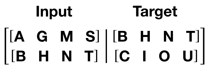
변수 덩어리는 트랜스포머 모델의 S 차원과 일치하는 0 차원에 해당합니다.
배치 차원 N 은 1 차원에 해당합니다.
bptt = 25
def get_batch(source, i):
    seq_len = min(bptt, len(source) - 1 - i)
    data = source[i:i+seq_len]
    target = source[i+1:i+1+seq_len].view(-1)
    # 파이프라인 병렬화를 위해 먼저 배치 차원이 필요합니다.
    return data.t(), target
모델 규모와 파이프 초기화#
파이프라인 병렬화를 활용한 대형 트랜스포머 모델 학습을 증명하기 위해서
트랜스포머 계층 규모를 적절히 확장시킵니다. 4096차원의 임베딩 벡터, 4096의 은닉 사이즈,
16개의 어텐션 헤드(attention head)와 총 12 개의 트랜스포머 계층
(nn.TransformerEncoderLayer)를 사용합니다. 이는 최대
1.4억 개의 파라미터를 갖는 모델을 생성합니다.
Pipe는 RRef 를 통해 RPC 프레임워크 에 의존하는데 이는 향후 호스트 파이프라인을 교차 확장할 수 있도록 하기 때문에 RPC 프레임워크를 초기화해야 합니다. 이때 RPC 프레임워크는 오직 하나의 하나의 worker로 초기화를 해야 하는데, 여러 GPU를 다루기 위해 프로세스 하나만 사용하고 있기 때문입니다.
그런 다음 파이프라인은 한 GPU에 8개의 트랜스포머와 다른 GPU에 8개의 트랜스포머 레이어로 초기화됩니다.
참고
효율성을 위해 Pipe 에 전달된 nn.Sequential 이
오직 두 개의 요소(2개의 GPU)로만 구성되도록 합니다. 이렇게 하면
Pipe가 두 개의 파티션에서만 작동하고
파티션 간 오버헤드를 피할 수 있습니다.
ntokens = len(vocab) # 단어 사전(어휘집)의 크기
emsize = 4096 # 임베딩 차원
nhid = 4096 # ``nn.TransformerEncoder`` 에서 순전파(feedforward) 신경망 모델의 차원
nlayers = 12 # ``nn.TransformerEncoder`` 내부의 ``nn.TransformerEncoderLayer`` 개수
nhead = 16 # Multihead Attention 모델의 헤드 개수
dropout = 0.2 # dropout 값

from torch.distributed import rpc
tmpfile = tempfile.NamedTemporaryFile()
rpc.init_rpc(
    name="worker",
    rank=0,
    world_size=1,
    rpc_backend_options=rpc.TensorPipeRpcBackendOptions(
        init_method="file://{}".format(tmpfile.name),
        # _transports와 _channels를 지정하는 것이 해결 방법이며
        # PyTorch 버전 >= 1.8.1 에서는 _transports와 _channels를
        # 지정하지 않아도 됩니다.
        _transports=["ibv", "uv"],
        _channels=["cuda_ipc", "cuda_basic"],
    )
)

num_gpus = 2
partition_len = ((nlayers - 1) // num_gpus) + 1

# 처음에 인코더를 추가합니다.
tmp_list = [Encoder(ntokens, emsize, dropout).cuda(0)]
module_list = []

# 필요한 모든 트랜스포머 블록들을 추가합니다.
for i in range(nlayers):
    transformer_block = TransformerEncoderLayer(emsize, nhead, nhid, dropout)
    if i != 0 and i % (partition_len) == 0:
        module_list.append(nn.Sequential(*tmp_list))
        tmp_list = []
    device = i // (partition_len)
    tmp_list.append(transformer_block.to(device))

# 마지막에 디코더를 추가합니다.
tmp_list.append(Decoder(ntokens, emsize).cuda(num_gpus - 1))
module_list.append(nn.Sequential(*tmp_list))

from torch.distributed.pipeline.sync import Pipe

# 파이프라인을 빌드합니다.
chunks = 8
model = Pipe(torch.nn.Sequential(*module_list), chunks = chunks)


def get_total_params(module: torch.nn.Module):
    total_params = 0
    for param in module.parameters():
        total_params += param.numel()
    return total_params

print ('Total parameters in model: {:,}'.format(get_total_params(model)))
모델 실행하기#
손실(loss)을 추적하기 위해 CrossEntropyLoss 가 적용되며, 옵티마이저(optimizer)로서 SGD 는 확률적 경사하강법(stochastic gradient descent method)을 구현합니다. 초기 학습률(learning rate)은 5.0로 설정됩니다. StepLR 는 에폭(epoch)에 따라서 학습률을 조절하는 데 사용됩니다. 학습하는 동안, 기울기 폭발(gradient exploding)을 방지하기 위해 모든 기울기를 함께 조정(scale)하는 함수 nn.utils.clip_grad_norm_ 을 이용합니다.
criterion = nn.CrossEntropyLoss()
lr = 5.0 # 학습률
optimizer = torch.optim.SGD(model.parameters(), lr=lr)
scheduler = torch.optim.lr_scheduler.StepLR(optimizer, 1.0, gamma=0.95)

import time
def train():
    model.train() # 훈련 모드로 전환
    total_loss = 0.
    start_time = time.time()
    ntokens = len(vocab)

    # 스크립트 실행 시간을 짧게 유지하기 위해서 50 배치만 학습합니다.
    nbatches = min(50 * bptt, train_data.size(0) - 1)

    for batch, i in enumerate(range(0, nbatches, bptt)):
        data, targets = get_batch(train_data, i)
        optimizer.zero_grad()
        # Pipe는 단일 호스트 내에 있고
        # forward 메서드로 반환된 ``RRef`` 프로세스는 이 노드에 국한되어 있기 때문에
        # ``RRef.local_value()`` 를 통해 간단히 찾을 수 있습니다.
        output = model(data).local_value()
        # 타겟을 파이프라인 출력이 있는
        # 장치로 옮겨야합니다.
        loss = criterion(output.view(-1, ntokens), targets.cuda(1))
        loss.backward()
        torch.nn.utils.clip_grad_norm_(model.parameters(), 0.5)
        optimizer.step()

        total_loss += loss.item()
        log_interval = 10
        if batch % log_interval == 0 and batch > 0:
            cur_loss = total_loss / log_interval
            elapsed = time.time() - start_time
            print('| epoch {:3d} | {:5d}/{:5d} batches | '
                  'lr {:02.2f} | ms/batch {:5.2f} | '
                  'loss {:5.2f} | ppl {:8.2f}'.format(
                    epoch, batch, nbatches // bptt, scheduler.get_lr()[0],
                    elapsed * 1000 / log_interval,
                    cur_loss, math.exp(cur_loss)))
            total_loss = 0
            start_time = time.time()

def evaluate(eval_model, data_source):
    eval_model.eval() # 평가 모드로 전환
    total_loss = 0.
    ntokens = len(vocab)
    # 스크립트 실행 시간을 짧게 유지하기 위해 50 배치만 평가합니다.
    nbatches = min(50 * bptt, data_source.size(0) - 1)
    with torch.no_grad():
        for i in range(0, nbatches, bptt):
            data, targets = get_batch(data_source, i)
            output = eval_model(data).local_value()
            output_flat = output.view(-1, ntokens)
            # 타겟을 파이프라인 출력이 있는
            # 장치로 옮겨야합니다.
            total_loss += len(data) * criterion(output_flat, targets.cuda(1)).item()
    return total_loss / (len(data_source) - 1)
에폭을 반복합니다. 만약 검증 오차(validation loss)가 지금까지 관찰한 것 중 최적이라면 모델을 저장합니다. 각 에폭 이후에 학습률을 조절합니다.
best_val_loss = float("inf")
epochs = 3 # 에폭 수
best_model = None

for epoch in range(1, epochs + 1):
    epoch_start_time = time.time()
    train()
    val_loss = evaluate(model, val_data)
    print('-' * 89)
    print('| end of epoch {:3d} | time: {:5.2f}s | valid loss {:5.2f} | '
          'valid ppl {:8.2f}'.format(epoch, (time.time() - epoch_start_time),
                                     val_loss, math.exp(val_loss)))
    print('-' * 89)

    if val_loss < best_val_loss:
        best_val_loss = val_loss
        best_model = model

    scheduler.step()
평가 데이터셋으로 모델 평가하기#
평가 데이터셋에서의 결과를 확인하기 위해 최고의 모델을 적용합니다.
test_loss = evaluate(best_model, test_data)
print('=' * 89)
print('| End of training | test loss {:5.2f} | test ppl {:8.2f}'.format(
    test_loss, math.exp(test_loss)))
print('=' * 89)
Total running time of the script: (0 minutes 0.119 seconds)
