


참고
Go to the end to download the full example code.
기초부터 시작하는 NLP: 문자-단위 RNN으로 이름 분류하기#
- Author: Sean Robertson
이 튜토리얼은 3부로 구성된 시리즈의 일부입니다:
여기에서는 단어를 분류하기 위해 기초적인 문자-단위의 순환 신경망(RNN, Recurrent Nueral Network)을 구축하고 학습할 예정입니다. 이 튜토리얼 및 이후 2개 튜토리얼인 기초부터 시작하는 NLP: 문자-단위 RNN으로 이름 생성하기 및 기초부터 시작하는 NLP: Sequence to Sequence 네트워크와 Attention을 이용한 번역 에서는 자연어 처리(NLP, Natural Language Processing) 분야에서 어떻게 데이터를 전처리하고 NLP 모델을 구축하는지를 밑바닥부터(from scratch) 설명합니다. 이를 위해 이 튜토리얼 시리즈에서는 NLP 모델링을 위한 데이터 전처리가 밑바닥(low-level)에서 어떻게 진행되는지 알 수 있습니다.
문자-단위 RNN은 단어를 문자의 연속으로 읽어 들여서 각 단계의 예측과 “은닉 상태(Hidden State)”를 출력하고, 다음 단계에 이전 단계의 은닉 상태를 전달합니다. 단어가 속한 클래스로 출력되도록 최종 예측으로 선택합니다.
구체적으로, 18개 언어로 된 수천 개의 성(姓)을 훈련시키고, 철자에 따라 이름이 어떤 언어인지 예측합니다.
Torch 준비#
하드웨어(CPU 또는 CUDA)에 맞춰 GPU 가속을 사용할 수 있도록 적절한 장치를 기본 장치로 설정합니다.
import torch

# Check if CUDA is available
device = torch.device('cpu')
if torch.cuda.is_available():
    device = torch.device('cuda')

torch.set_default_device(device)
print(f"Using device = {torch.get_default_device()}")
Using device = cuda:0
데이터 준비#
여기 에서 데이터를 다운로드 받고 현재 디렉토리에 압축을 풉니다.
data/names 디렉토리에는 [Language].txt 라는 18 개의 텍스트 파일이 있습니다.
각 파일에는 한 줄에 하나의 이름이 포함되어 있으며 대부분 로마자로 되어 있습니다.
(하지만 유니코드에서 ASCII로 변환은 해야 합니다)
첫번째 단계는 데이터를 정의하고 정리하는 것입니다. 초기에는 유니코드를 일반 ASCII로 변환하여 RNN 입력 레이어를 제한해야 합니다. 이는 유니코드 문자열을 ASCII로 변환하고 허용된 문자의 작은 집합만을 허용하여 이루어집니다.
import string
import unicodedata

# "_" 를 사용하여 어휘집(Vocabulary)에 없는 문자를 표현할 수 있습니다. 즉, 모델에서 처리하지 않는 모든 문자를 표현할 수 있습니다.
allowed_characters = string.ascii_letters + " .,;'" + "_"
n_letters = len(allowed_characters)

# 유니코드 문자열을 일반 ASCII로 변환하기: https://stackoverflow.com/a/518232/2809427
def unicodeToAscii(s):
    return ''.join(
        c for c in unicodedata.normalize('NFD', s)
        if unicodedata.category(c) != 'Mn'
        and c in allowed_characters
    )
유니코드 알파벳 이름을 일반 ASCII로 변환하는 예시입니다. 이렇게 하면 입력 레이어를 단순화할 수 있습니다.
print (f"converting 'Ślusàrski' to {unicodeToAscii('Ślusàrski')}")
converting 'Ślusàrski' to Slusarski
이름을 Tensor로 변경#
이제 모든 이름을 체계화했으므로, 이를 활용하기 위해 Tensor로 변환해야 합니다.
하나의 문자를 표현하기 위해 크기가 <1 x n_letters> 인
“One-Hot 벡터”를 사용합니다. One-Hot 벡터는 현재 문자의
주소에는 1이, 그 외 나머지 주소에는 0이 채워진 벡터입니다.
예시 "b" = <0 1 0 0 0 ...> .
단어를 만들기 위해 One-Hot 벡터들을 2차원 행렬
<line_length x 1 x n_letters> 에 결합시킵니다.
위에서 보이는 추가적인 1차원은 PyTorch에서 모든 것이 배치(batch)에 있다고 가정하기 때문에 발생합니다. 여기서는 배치 크기 1을 사용하고 있습니다.
# .. note::
#    역자 주: One-Hot 벡터는 언어 및 범주형 데이터를 다룰 때 주로 사용하며,
#    단어, 글자 등을 벡터로 표현할 때 단어, 글자 사이의 상관 관계를 미리 알 수 없을 경우,
#    One-Hot으로 표현하여 서로 직교한다고 가정하고 학습을 시작합니다.
#    이와 동일하게, 상관 관계를 알 수 없는 다른 데이터의 경우에도 One-Hot 벡터를 활용할 수 있습니다.
#

import torch

# all_letters 로 문자의 주소 찾기, 예시 "a" = 0
def letterToIndex(letter):
    # 모델이 모르는 글자를 만나면, 어휘집에 존재하지 않는 문자("_")를 반환합니다.
    if letter not in allowed_characters:
        return allowed_characters.find("_")
    else:
        return allowed_characters.find(letter)

# 검증을 위해서 한 개의 문자를 <1 x n_letters> Tensor로 변환
def letterToTensor(letter):
    tensor = torch.zeros(1, n_letters)
    tensor[0][letterToIndex(letter)] = 1
    return tensor

# 한 줄(이름)을  <line_length x 1 x n_letters>,
# 또는 One-Hot 문자 벡터의 Array로 변경
def lineToTensor(line):
    tensor = torch.zeros(len(line), 1, n_letters)
    for li, letter in enumerate(line):
        tensor[li][0][letterToIndex(letter)] = 1
    return tensor

print(letterToTensor('J'))

print(lineToTensor('Jones').size())
tensor([[0., 0., 0., 0., 0., 0., 0., 0., 0., 0., 0., 0., 0., 0., 0., 0., 0., 0.,
         0., 0., 0., 0., 0., 0., 0., 0., 0., 0., 0., 0., 0., 0., 0., 0., 0., 1.,
         0., 0., 0., 0., 0., 0., 0., 0., 0., 0., 0., 0., 0., 0., 0., 0., 0., 0.,
         0., 0., 0., 0.]], device='cuda:0')
torch.Size([5, 1, 58])
Here are some examples of how to use lineToTensor() for a single and multiple character string.
print (f"The letter 'a' becomes {lineToTensor('a')}") #notice that the first position in the tensor = 1
print (f"The name 'Ahn' becomes {lineToTensor('Ahn')}") #notice 'A' sets the 27th index to 1
The letter 'a' becomes tensor([[[1., 0., 0., 0., 0., 0., 0., 0., 0., 0., 0., 0., 0., 0., 0., 0., 0.,
          0., 0., 0., 0., 0., 0., 0., 0., 0., 0., 0., 0., 0., 0., 0., 0., 0.,
          0., 0., 0., 0., 0., 0., 0., 0., 0., 0., 0., 0., 0., 0., 0., 0., 0.,
          0., 0., 0., 0., 0., 0., 0.]]], device='cuda:0')
The name 'Ahn' becomes tensor([[[0., 0., 0., 0., 0., 0., 0., 0., 0., 0., 0., 0., 0., 0., 0., 0., 0.,
          0., 0., 0., 0., 0., 0., 0., 0., 0., 1., 0., 0., 0., 0., 0., 0., 0.,
          0., 0., 0., 0., 0., 0., 0., 0., 0., 0., 0., 0., 0., 0., 0., 0., 0.,
          0., 0., 0., 0., 0., 0., 0.]],

        [[0., 0., 0., 0., 0., 0., 0., 1., 0., 0., 0., 0., 0., 0., 0., 0., 0.,
          0., 0., 0., 0., 0., 0., 0., 0., 0., 0., 0., 0., 0., 0., 0., 0., 0.,
          0., 0., 0., 0., 0., 0., 0., 0., 0., 0., 0., 0., 0., 0., 0., 0., 0.,
          0., 0., 0., 0., 0., 0., 0.]],

        [[0., 0., 0., 0., 0., 0., 0., 0., 0., 0., 0., 0., 0., 1., 0., 0., 0.,
          0., 0., 0., 0., 0., 0., 0., 0., 0., 0., 0., 0., 0., 0., 0., 0., 0.,
          0., 0., 0., 0., 0., 0., 0., 0., 0., 0., 0., 0., 0., 0., 0., 0., 0.,
          0., 0., 0., 0., 0., 0., 0.]]], device='cuda:0')
Congratulations, you have built the foundational tensor objects for this learning task! You can use a similar approach for other RNN tasks with text.
Next, we need to combine all our examples into a dataset so we can train, test and validate our models. For this,
we will use the Dataset and DataLoader classes
to hold our dataset. Each Dataset needs to implement three functions: __init__, __len__, and __getitem__.
from io import open
import glob
import os
import time

import torch
from torch.utils.data import Dataset

class NamesDataset(Dataset):

    def __init__(self, data_dir):
        self.data_dir = data_dir #for provenance of the dataset
        self.load_time = time.localtime #for provenance of the dataset
        labels_set = set() #set of all classes

        self.data = []
        self.data_tensors = []
        self.labels = []
        self.labels_tensors = []

        #read all the ``.txt`` files in the specified directory
        text_files = glob.glob(os.path.join(data_dir, '*.txt'))
        for filename in text_files:
            label = os.path.splitext(os.path.basename(filename))[0]
            labels_set.add(label)
            lines = open(filename, encoding='utf-8').read().strip().split('\n')
            for name in lines:
                self.data.append(name)
                self.data_tensors.append(lineToTensor(name))
                self.labels.append(label)

        #Cache the tensor representation of the labels
        self.labels_uniq = list(labels_set)
        for idx in range(len(self.labels)):
            temp_tensor = torch.tensor([self.labels_uniq.index(self.labels[idx])], dtype=torch.long)
            self.labels_tensors.append(temp_tensor)

    def __len__(self):
        return len(self.data)

    def __getitem__(self, idx):
        data_item = self.data[idx]
        data_label = self.labels[idx]
        data_tensor = self.data_tensors[idx]
        label_tensor = self.labels_tensors[idx]

        return label_tensor, data_tensor, data_label, data_item
Here we can load our example data into the NamesDataset
alldata = NamesDataset("data/names")
print(f"loaded {len(alldata)} items of data")
print(f"example = {alldata[0]}")
loaded 20074 items of data
example = (tensor([1], device='cuda:0'), tensor([[[0., 0., 0., 0., 0., 0., 0., 0., 0., 0., 0., 0., 0., 0., 0., 0., 0.,
          0., 0., 0., 0., 0., 0., 0., 0., 0., 1., 0., 0., 0., 0., 0., 0., 0.,
          0., 0., 0., 0., 0., 0., 0., 0., 0., 0., 0., 0., 0., 0., 0., 0., 0.,
          0., 0., 0., 0., 0., 0., 0.]],

        [[0., 1., 0., 0., 0., 0., 0., 0., 0., 0., 0., 0., 0., 0., 0., 0., 0.,
          0., 0., 0., 0., 0., 0., 0., 0., 0., 0., 0., 0., 0., 0., 0., 0., 0.,
          0., 0., 0., 0., 0., 0., 0., 0., 0., 0., 0., 0., 0., 0., 0., 0., 0.,
          0., 0., 0., 0., 0., 0., 0.]],

        [[0., 1., 0., 0., 0., 0., 0., 0., 0., 0., 0., 0., 0., 0., 0., 0., 0.,
          0., 0., 0., 0., 0., 0., 0., 0., 0., 0., 0., 0., 0., 0., 0., 0., 0.,
          0., 0., 0., 0., 0., 0., 0., 0., 0., 0., 0., 0., 0., 0., 0., 0., 0.,
          0., 0., 0., 0., 0., 0., 0.]],

        [[1., 0., 0., 0., 0., 0., 0., 0., 0., 0., 0., 0., 0., 0., 0., 0., 0.,
          0., 0., 0., 0., 0., 0., 0., 0., 0., 0., 0., 0., 0., 0., 0., 0., 0.,
          0., 0., 0., 0., 0., 0., 0., 0., 0., 0., 0., 0., 0., 0., 0., 0., 0.,
          0., 0., 0., 0., 0., 0., 0.]],

        [[0., 0., 0., 0., 0., 0., 0., 0., 0., 0., 0., 0., 0., 0., 0., 0., 0.,
          0., 1., 0., 0., 0., 0., 0., 0., 0., 0., 0., 0., 0., 0., 0., 0., 0.,
          0., 0., 0., 0., 0., 0., 0., 0., 0., 0., 0., 0., 0., 0., 0., 0., 0.,
          0., 0., 0., 0., 0., 0., 0.]]], device='cuda:0'), 'English', 'Abbas')
Using the dataset object allows us to easily split the data into train and test sets. Here we create a 80/20
split but the torch.utils.data has more useful utilities. Here we specify a generator since we need to use the
same device as PyTorch defaults to above.
train_set, test_set = torch.utils.data.random_split(alldata, [.85, .15], generator=torch.Generator(device=device).manual_seed(2024))

print(f"train examples = {len(train_set)}, validation examples = {len(test_set)}")
train examples = 17063, validation examples = 3011
Now we have a basic dataset containing 20074 examples where each example is a pairing of label and name. We have also split the dataset into training and testing so we can validate the model that we build.
네트워크 생성#
Autograd 전에, Torch에서 RNN(recurrent neural network) 생성은 여러 시간 단계 걸쳐서 계층의 매개변수를 복제하는 작업을 포함합니다. 계층은 은닉 상태와 변화도(Gradient)를 가지며, 이제 이것들은 그래프 자체에서 완전히 처리됩니다. 이는 feed-forward 계층과 같은 매우 “순수한” 방법으로 RNN을 구현할 수 있음을 의미합니다.
참고
역자 주: 여기서는 학습 목적으로 nn.RNN 대신 직접 RNN을 사용합니다.
이 RNN 모듈은 “기본(vanilla)적인 RNN”을 구현하며, 입력과 은닉 상태(hidden state),
그리고 출력 뒤 동작하는 LogSoftmax 계층이 있는 3개의 선형 계층만을 가집니다.
This CharRNN class implements an RNN with three components.
First, we use the nn.RNN implementation.
Next, we define a layer that maps the RNN hidden layers to our output. And finally, we apply a softmax function. Using nn.RNN
leads to a significant improvement in performance, such as cuDNN-accelerated kernels, versus implementing
each layer as a nn.Linear. It also simplifies the implementation in forward().
import torch.nn as nn
import torch.nn.functional as F

class CharRNN(nn.Module):
    def __init__(self, input_size, hidden_size, output_size):
        super(CharRNN, self).__init__()

        self.rnn = nn.RNN(input_size, hidden_size)
        self.h2o = nn.Linear(hidden_size, output_size)
        self.softmax = nn.LogSoftmax(dim=1)

    def forward(self, line_tensor):
        rnn_out, hidden = self.rnn(line_tensor)
        output = self.h2o(hidden[0])
        output = self.softmax(output)

        return output
We can then create an RNN with 58 input nodes, 128 hidden nodes, and 18 outputs:
n_hidden = 128
rnn = CharRNN(n_letters, n_hidden, len(alldata.labels_uniq))
print(rnn)
CharRNN(
  (rnn): RNN(58, 128)
  (h2o): Linear(in_features=128, out_features=18, bias=True)
  (softmax): LogSoftmax(dim=1)
)
After that we can pass our Tensor to the RNN to obtain a predicted output. Subsequently,
we use a helper function, label_from_output, to derive a text label for the class.
def label_from_output(output, output_labels):
    top_n, top_i = output.topk(1)
    label_i = top_i[0].item()
    return output_labels[label_i], label_i

input = lineToTensor('Albert')
output = rnn(input) #this is equivalent to ``output = rnn.forward(input)``
print(output)
print(label_from_output(output, alldata.labels_uniq))
tensor([[-2.9395, -3.0940, -2.8990, -2.9367, -2.8716, -2.7607, -2.9501, -2.8651,
         -2.8425, -2.8339, -2.8015, -2.9372, -2.9002, -2.9046, -2.8947, -2.8643,
         -2.9327, -2.8415]], device='cuda:0', grad_fn=<LogSoftmaxBackward0>)
('Greek', 5)
학습#
신경망 학습#
이제 이 네트워크를 학습하는 데 필요한 예시(학습 데이터)를 보여주고 추정합니다. 만일 틀렸다면 알려 줍니다.
We do this by defining a train() function which trains the model on a given dataset using minibatches. RNNs
RNNs are trained similarly to other networks; therefore, for completeness, we include a batched training method here.
The loop (for i in batch) computes the losses for each of the items in the batch before adjusting the
weights. This operation is repeated until the number of epochs is reached.
import random
import numpy as np

def train(rnn, training_data, n_epoch = 10, n_batch_size = 64, report_every = 50, learning_rate = 0.2, criterion = nn.NLLLoss()):
    """
    Learn on a batch of training_data for a specified number of iterations and reporting thresholds
    """
    # Keep track of losses for plotting
    current_loss = 0
    all_losses = []
    rnn.train()
    optimizer = torch.optim.SGD(rnn.parameters(), lr=learning_rate)

    start = time.time()
    print(f"training on data set with n = {len(training_data)}")

    for iter in range(1, n_epoch + 1):
        rnn.zero_grad() # clear the gradients

        # create some minibatches
        # we cannot use dataloaders because each of our names is a different length
        batches = list(range(len(training_data)))
        random.shuffle(batches)
        batches = np.array_split(batches, len(batches) //n_batch_size )

        for idx, batch in enumerate(batches):
            batch_loss = 0
            for i in batch: #for each example in this batch
                (label_tensor, text_tensor, label, text) = training_data[i]
                output = rnn.forward(text_tensor)
                loss = criterion(output, label_tensor)
                batch_loss += loss

            # optimize parameters
            batch_loss.backward()
            nn.utils.clip_grad_norm_(rnn.parameters(), 3)
            optimizer.step()
            optimizer.zero_grad()

            current_loss += batch_loss.item() / len(batch)

        all_losses.append(current_loss / len(batches) )
        if iter % report_every == 0:
            print(f"{iter} ({iter / n_epoch:.0%}): \t average batch loss = {all_losses[-1]}")
        current_loss = 0

    return all_losses
We can now train a dataset with minibatches for a specified number of epochs. The number of epochs for this example is reduced to speed up the build. You can get better results with different parameters.
start = time.time()
all_losses = train(rnn, train_set, n_epoch=27, learning_rate=0.15, report_every=5)
end = time.time()
print(f"training took {end-start}s")
training on data set with n = 17063
5 (19%):         average batch loss = 0.8897688550849814
10 (37%):        average batch loss = 0.6987682116383276
15 (56%):        average batch loss = 0.5792883489287404
20 (74%):        average batch loss = 0.4965955759470279
25 (93%):        average batch loss = 0.43885368771157285
training took 270.788941860199s
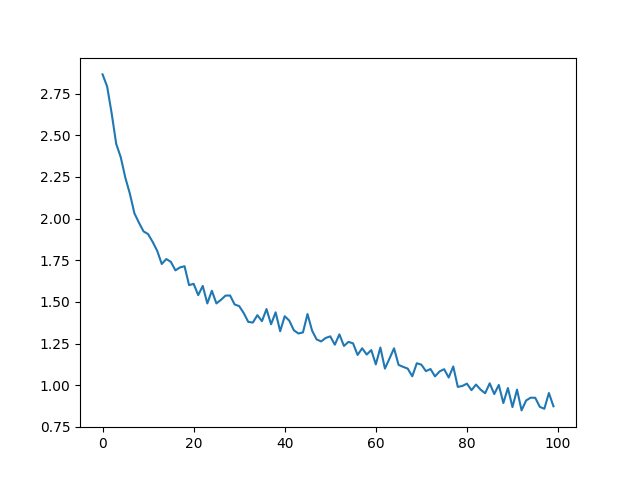
결과 도식화#
all_losses 를 이용한 손실 도식화는
네트워크의 학습을 보여줍니다:
import matplotlib.pyplot as plt
import matplotlib.ticker as ticker

plt.figure()
plt.plot(all_losses)
plt.show()
결과 평가#
네트워크가 다른 카테고리에서 얼마나 잘 작동하는지 보기 위해
모든 실제 언어(행)가 네트워크에서 어떤 언어로 추측(열)되는지 나타내는
혼란 행렬(confusion matrix)을 만듭니다. 혼란 행렬을 계산하기 위해
evaluate() 로 많은 수의 샘플을 네트워크에 실행합니다.
evaluate() 은 train () 과 역전파를 빼면 동일합니다.
def evaluate(rnn, testing_data, classes):
    confusion = torch.zeros(len(classes), len(classes))

    rnn.eval() #set to eval mode
    with torch.no_grad(): # do not record the gradients during eval phase
        for i in range(len(testing_data)):
            (label_tensor, text_tensor, label, text) = testing_data[i]
            output = rnn(text_tensor)
            guess, guess_i = label_from_output(output, classes)
            label_i = classes.index(label)
            confusion[label_i][guess_i] += 1

    # Normalize by dividing every row by its sum
    for i in range(len(classes)):
        denom = confusion[i].sum()
        if denom > 0:
            confusion[i] = confusion[i] / denom

    # Set up plot
    fig = plt.figure()
    ax = fig.add_subplot(111)
    cax = ax.matshow(confusion.cpu().numpy()) #numpy uses cpu here so we need to use a cpu version
    fig.colorbar(cax)

    # Set up axes
    ax.set_xticks(np.arange(len(classes)), labels=classes, rotation=90)
    ax.set_yticks(np.arange(len(classes)), labels=classes)

    # Force label at every tick
    ax.xaxis.set_major_locator(ticker.MultipleLocator(1))
    ax.yaxis.set_major_locator(ticker.MultipleLocator(1))

    # sphinx_gallery_thumbnail_number = 2
    plt.show()


evaluate(rnn, test_set, classes=alldata.labels_uniq)
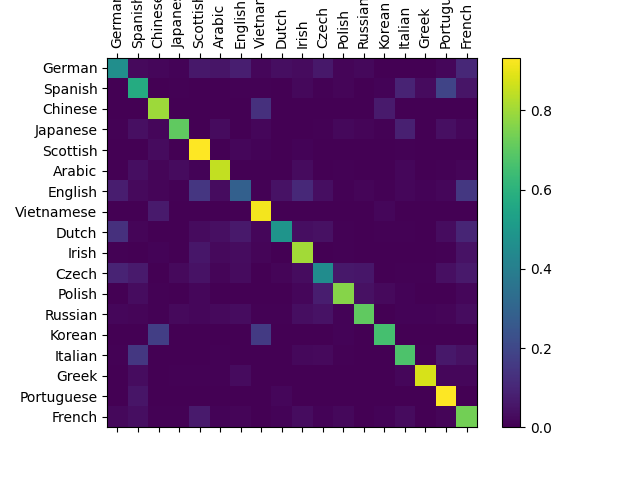
주축에서 벗어난 밝은 점을 선택하여 잘못 추측한 언어를 표시할 수 있습니다. 예를 들어 한국어는 중국어로 이탈리아어로 스페인어로. 그리스어는 매우 잘되는 것으로 영어는 매우 나쁜 것으로 보입니다. (다른 언어들과의 중첩 때문으로 추정)
연습#
Get better results with a bigger and/or better shaped network
Adjust the hyperparameters to enhance performance, such as changing the number of epochs, batch size, and learning rate
Try the
nn.LSTMandnn.GRUlayersModify the size of the layers, such as increasing or decreasing the number of hidden nodes or adding additional linear layers
Combine multiple of these RNNs as a higher level network
“line -> label” 의 다른 데이터 집합으로 시도해 보십시오, 예를 들어:
단어 -> 언어
이름 -> 성별
캐릭터 이름 -> 작가
페이지 제목 -> 블로그 또는 서브레딧
더 크고 더 나은 모양의 네트워크로 더 나은 결과를 얻으십시오.
더 많은 선형 계층을 추가해 보십시오.
nn.LSTM과nn.GRU계층을 추가해 보십시오.위와 같은 RNN 여러 개를 상위 수준 네트워크로 결합해 보십시오.
Total running time of the script: (4 minutes 41.329 seconds)
